下記の試行をしました:
- t-SNE、UMAPを試行。MNIST 8x8手書き数字画像1797枚を使用。
- それぞれ分けられた分布の中にある数字の形の傾向を調べる。
結果:
- 1の画像は3つの分布に分かれて、それぞれ、かぎがない棒だけの1の形状のタイプ、上にかぎのある1の形状のタイプ、左に傾けて崩して書く1の形状のタイプ、に分かれる様子が見られる。1の中でも傾向によりさらに分割され、良い分別の性能。
- 3の画像は1つの分布に集まるが、その中でも幅が細く書かれた3は右側へ、幅いっぱいに広げて書かれた3は左側へ、傾向によりさらに分割され、良い分別の性能。その他の数字でも同様の傾向が見られる。
更に下記の試行を行いました: (画像サイズ大、枚数増加)
参照したもの:
ライブラリをLoad
import numpy as np
import matplotlib.pyplot as plt
データをLoad
# sec: load

from sklearn.datasets import load_digits
digits = load_digits()
print(digits.data.shape)
print(digits.target.shape)
print(digits.images.shape)
(1797, 64)
(1797,)
(1797, 8, 8)
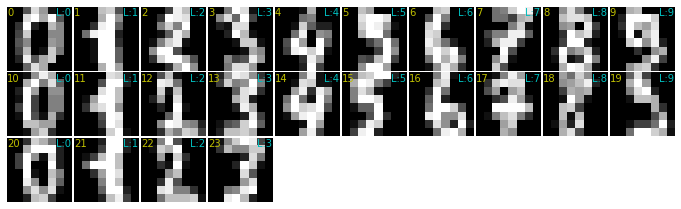
# sec: MNISTの画像をグリッド状に描画
def draw_digits(i_list, n_grid=(10, 10), annosize=10, figsize=(12, 12)):
# assume: i_listは画像配列の番号をリストに入れたもの、annosize=Noneで画像列番と正解ラベルを非表示
images = digits.images
labels =digits.target
fig = None
i_ax = 0
for i_img in i_list:
if fig is None or i_ax >= n_grid[0] * n_grid[1]:
fig = plt.figure(figsize=figsize)
plt.subplots_adjust(hspace=0.02, wspace=0)
i_ax = 0
i_ax += 1
ax = fig.add_subplot(n_grid[0], n_grid[1], i_ax)
if i_img is None:
ax.axis('off')
continue
ax.imshow(images[i_img], cmap='gray', interpolation='none')
if annosize is not None: # if: 画像列番と正解ラベルを追記
ax.annotate("%d" % i_img,
xy=(0, 0.98), xycoords='axes fraction', ha='left', va='top', color='y', fontsize=annosize)
ax.annotate("L:%d" % labels[i_img],
xy=(1, 0.98), xycoords='axes fraction', ha='right', va='top', color='c', fontsize=annosize)
ax.axis('off')
plt.show()
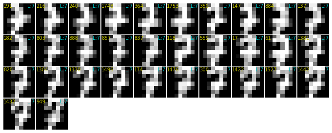
draw_digits(list(range(24)))
t-SNEを実行
from sklearn.manifold import TSNE
# sec: 実行

model = TSNE(n_components=2) # 2軸へ次元圧縮
res = model.fit_transform(digits.data)
print(res.shape)
(1797, 2)
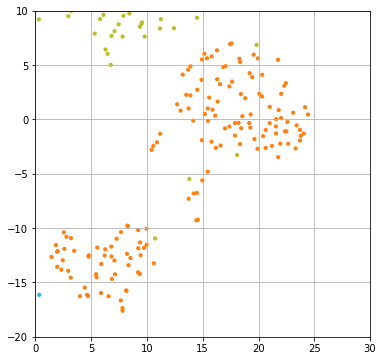
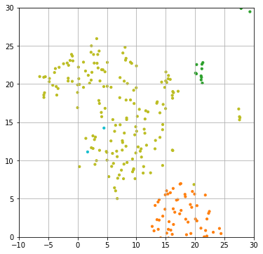
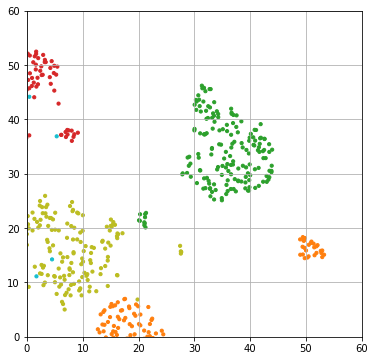
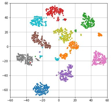
# sec: 結果の描画
import matplotlib.cm as cm
plt.figure(figsize=(12, 12))
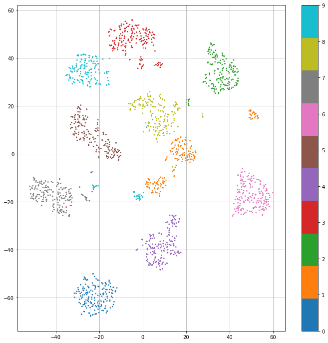
plt.scatter(res[:,0], res[:,1], s=3, c=digits.target, cmap=cm.tab10)
plt.colorbar()
plt.grid()
plt.show()
結果のグループを調べる
# sec: 結果を保存 毎回実行で変わる為

import pickle
with open("./results/2003 t-SNE/res-tsne-1.pickle", 'wb') as file:
    pickle.dump(res, file)
# sec: 結果を読み込み 前回の続きから

import pickle
with open("./results/2003 t-SNE/res-tsne-1.pickle", 'rb') as file:
    res = pickle.load(file)
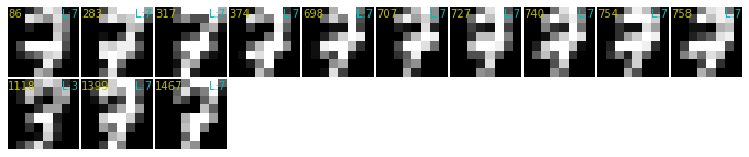
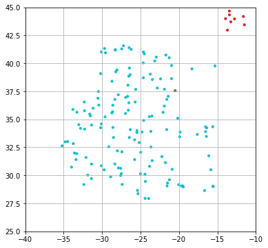
7の中の3を調べる
# sec: 7の中の3を調べる →1118番目のデータ ⇒確かに似ているもの同士が集まっている、解像度が低すぎる

import matplotlib.cm as cm
plt.scatter(res[:, 0], res[:, 1], s=10, c=digits.target, cmap=cm.tab10)
plt.axis([-50, -30, -30, -10]); plt.grid(); plt.show()
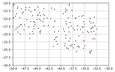
i_list = np.where((-37.5 < res[:, 0]) & (res[:, 0] < -32.5) & (-25 < res[:, 1]) & (res[:, 1] < -20))[0]
i_list
array([  86,  283,  317,  374,  698,  707,  727,  740,  754,  758, 1118,
       1399, 1467], dtype=int64)
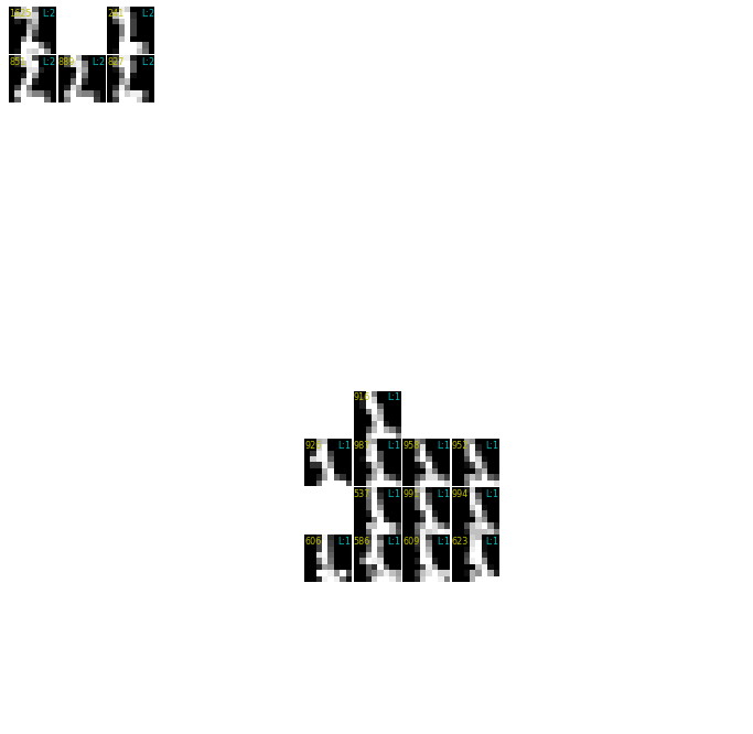
draw_digits(i_list)
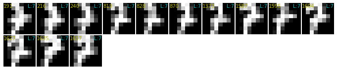
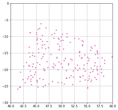
7の集団の下側を調べる
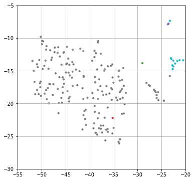
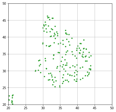
# sec: 7の集団の下側を調べる ⇒似ているか。やや丸みのない7が集まっている模様。

plt.scatter(res[:, 0], res[:, 1], s=10, c=digits.target, cmap=cm.tab10)
plt.axis([-60, -40, -30, -0]); plt.grid(); plt.show()
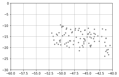
i_list = np.where((-55 < res[:, 0]) & (res[:, 0] < -50) & (-20 < res[:, 1]) & (res[:, 1] < -10))[0]
i_list
array([ 191,  216,  240,  819,  828,  870, 1373, 1587, 1595, 1604, 1627,
       1635, 1657], dtype=int64)
draw_digits(i_list)
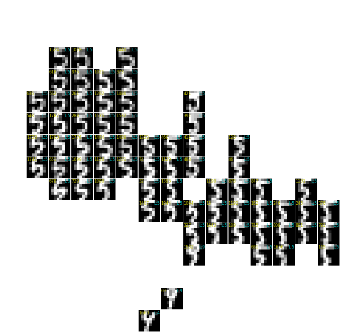
7の集団の横方向の画像を並べて変化を見る
# sec: 7の集団の横方向の画像を並べて変化を見る

i_list = np.where((-60 < res[:, 0]) & (res[:, 0] < -30) & (-20 < res[:, 1]) & (res[:, 1] < -18))[0]
i_list
array([  17,   61,  118,  137,  147,  174,  182,  191,  216,  240,  300,
        350,  364,  559,  803,  820,  837,  857,  884,  888,  949, 1304,
       1330, 1381, 1422, 1432, 1442, 1476, 1496, 1527, 1748, 1753],
      dtype=int64)
i_list = i_list[np.argsort(res[i_list, 0])] # x方向でソート
i_list
array([ 191,  216,  240, 1748,  364, 1753,  350,  147,  884,  137,  182,
        803,  888,  857,  837,  118,  559,   17,   61, 1381,  820, 1304,
       1330, 1496,  174, 1476,  300, 1422, 1527, 1442, 1432,  949],
      dtype=int64)
draw_digits(i_list)
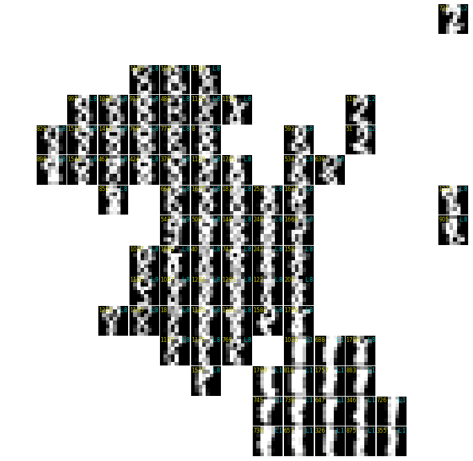
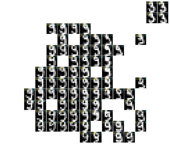
分布の位置に画像を当てはめて格子状に表示
def draw_digits_at_tsne(res, x_min, x_max, y_min, y_max,
n_grid=(15, 15), annosize=8, figsize=(12, 12)):
x_pitch = (x_max - x_min) / n_grid[1]
y_pitch = (y_max - y_min) / n_grid[0]
i_draw_list = []
for i_y in range(n_grid[0]):
y_i = y_max - y_pitch * i_y - y_pitch/2 # 格子中央点
for i_x in range(n_grid[1]):
x_i = x_min + x_pitch * i_x + x_pitch/2 # 格子中央点
i_list = np.where((x_i-x_pitch/2 < res[:, 0]) & (res[:, 0] < x_i+x_pitch/2) & \
(y_i-y_pitch/2 < res[:, 1]) & (res[:, 1] < y_i+y_pitch/2))[0] # 格子内の点を集める
res_i = res[i_list, :]
if len(res_i) == 0: # if: 格子内に点なし
i_draw_list.append(None)
continue
r2_i = ((res_i[:, 0] - x_i) / x_pitch)**2 + ((res_i[:, 1] - y_i) / y_pitch)**2 # 格子中央と点との距離
i_min = i_list[np.argmin(r2_i)] # 格子中央に最も近い点
i_draw_list.append(i_min)
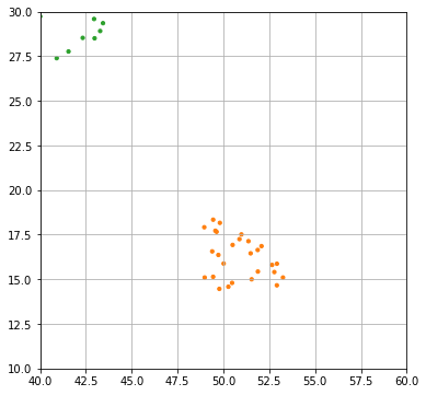
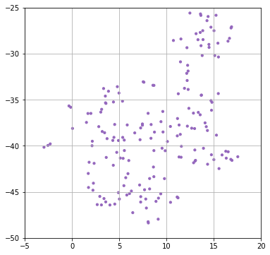
plt.figure(figsize=(6, 6))
plt.scatter(res[:, 0], res[:, 1], s=10, c=digits.target, cmap=cm.tab10) # 指定範囲内の点の分布を描画
plt.axis([x_min, x_max, y_min, y_max]); plt.grid(); plt.show()
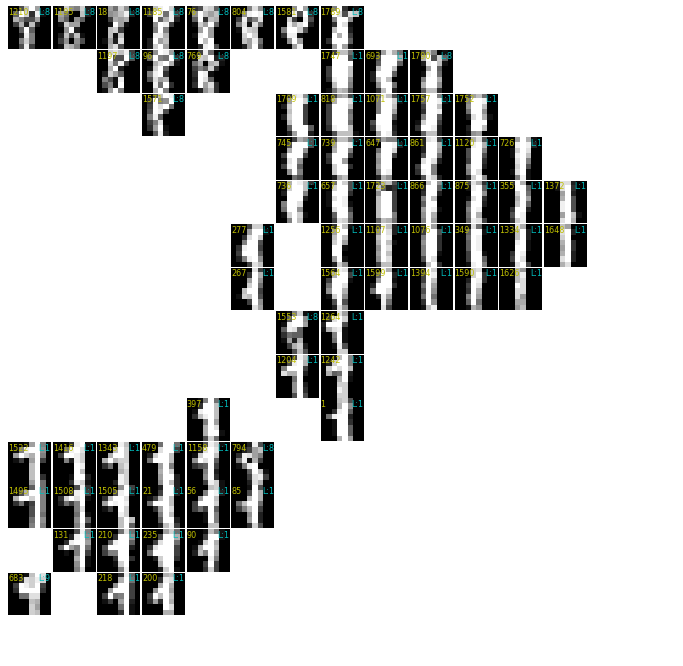
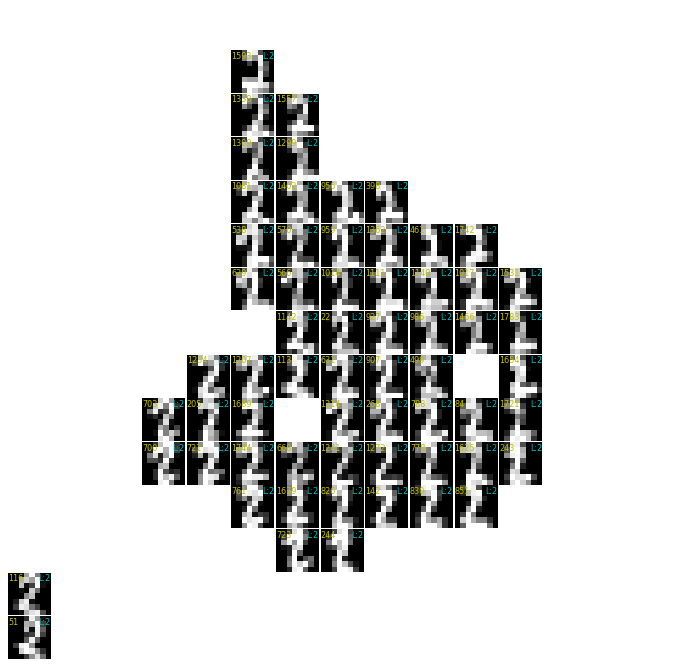
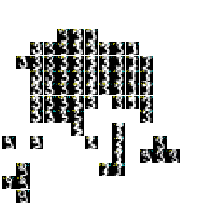
draw_digits(i_draw_list, n_grid=n_grid, annosize=annosize, figsize=figsize)
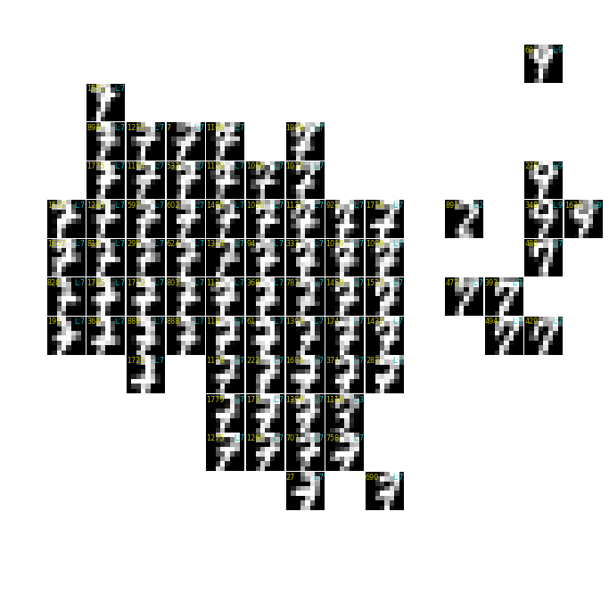
draw_digits_at_tsne(res, -55, -20, -30, -5)
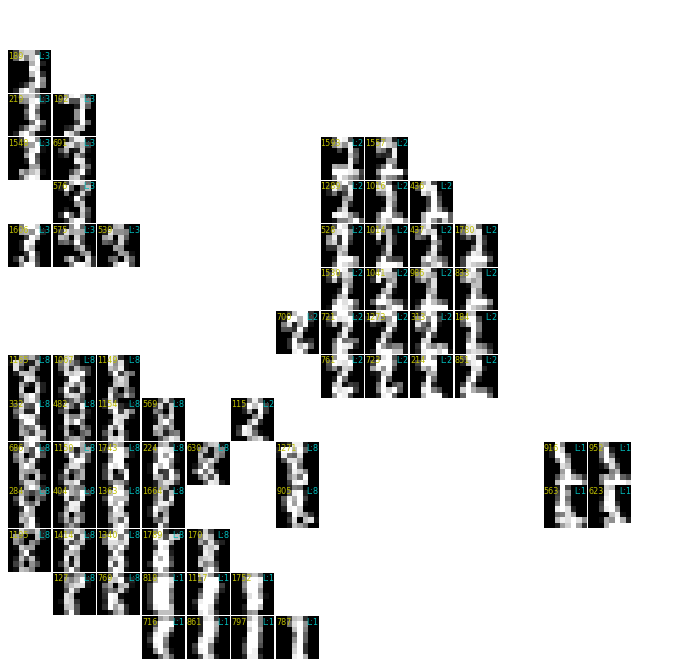
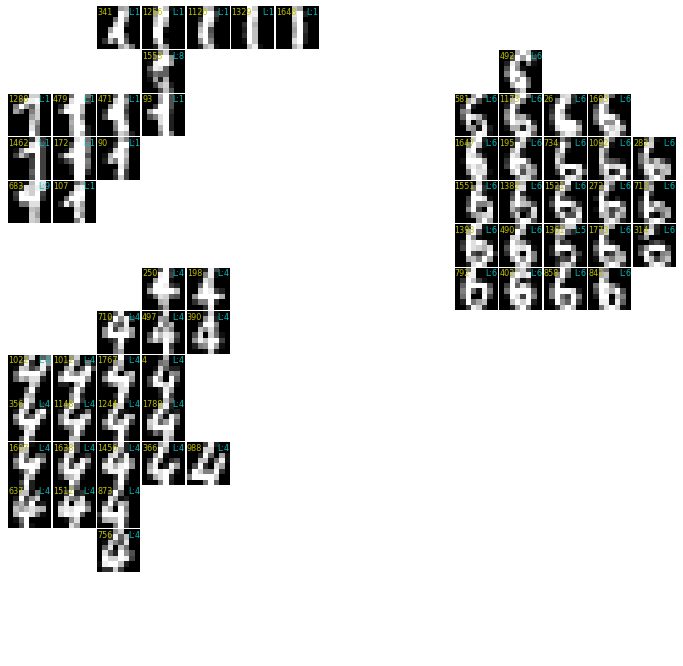
各数字の集団の分布状況を描画
# sec: 各数字の集団の分布状況を描画
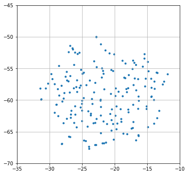
draw_digits_at_tsne(res, -35, -10, -70, -45) # 0周り
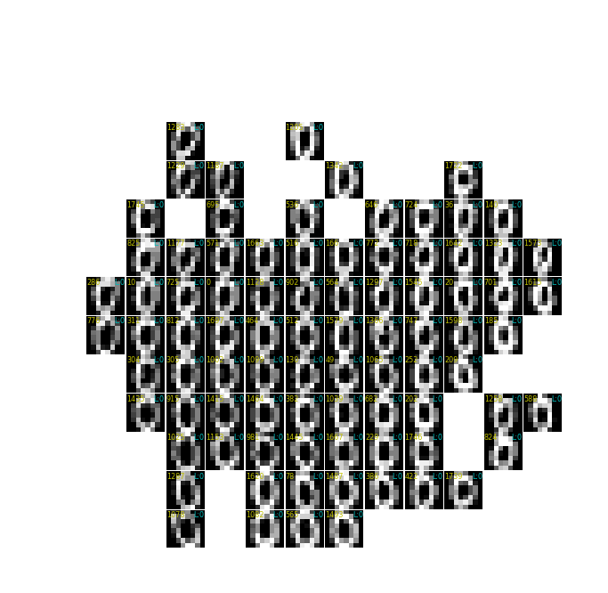
draw_digits_at_tsne(res, 0, 30, -20, 10) # 1周り
draw_digits_at_tsne(res, 40, 60, 10, 30) # 1周り
draw_digits_at_tsne(res, 20, 50, 20, 50) # 2周り
draw_digits_at_tsne(res, -20, 15, 30, 60) # 3周り
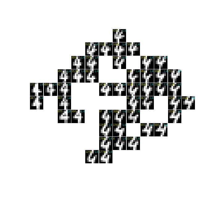
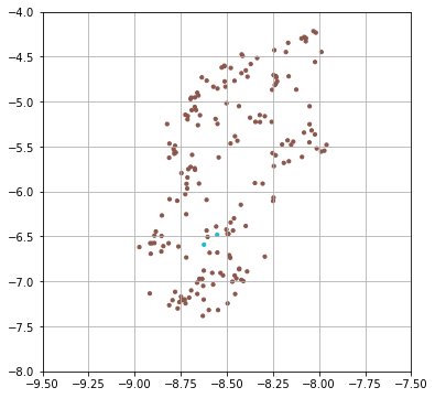
draw_digits_at_tsne(res, -5, 20, -50, -25) # 4周り
draw_digits_at_tsne(res, -35, -10, -10, 25) # 5周り
draw_digits_at_tsne(res, 40, 60, -30, 0) # 6周り

draw_digits_at_tsne(res, -55, -20, -30, -5) # 7周り


draw_digits_at_tsne(res, -10, 30, 0, 30) # 8周り
draw_digits_at_tsne(res, -40, -10, 25, 45) # 9周り
やや広めに分布状況を描画
# sec: やや広めに分布状況を描画

draw_digits_at_tsne(res, -40, 0, 0, 60) # 左上半面
draw_digits_at_tsne(res, 0, 60, 0, 60) # 右上半面
draw_digits_at_tsne(res, -60, 0, -70, 0) # 左下半面
draw_digits_at_tsne(res, 0, 60, -60, 0) # 右下半面
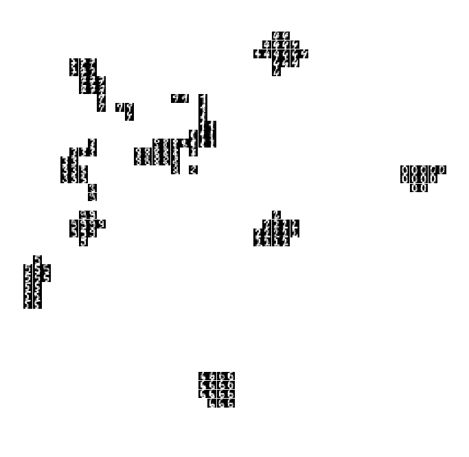
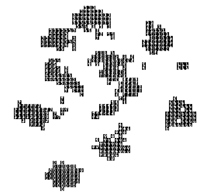
全体の分布状況を描画
draw_digits_at_tsne(res, -60, 60, -70, 60, n_grid=(50, 50), annosize=None)
UMAPを試す
t-SNEの試行の中で作った描画用の関数を使用。
!pip3 install umap-learn
Collecting umap-learn
  Downloading https://files.pythonhosted.org/packages/ad/92/36bac74962b424870026cb0b42cec3d5b6f4afa37d81818475d8762f9255/umap-learn-0.3.10.tar.gz (40kB)
Requirement already satisfied: numpy>=1.13 in ...\software\wpy64-3741\python-3.7.4.amd64\lib\site-packages (from umap-learn) (1.16.5+mkl)
Requirement already satisfied: scikit-learn>=0.16 in ...\software\wpy64-3741\python-3.7.4.amd64\lib\site-packages (from umap-learn) (0.21.3)
Requirement already satisfied: scipy>=0.19 in ...\software\wpy64-3741\python-3.7.4.amd64\lib\site-packages (from umap-learn) (1.3.1)
Requirement already satisfied: numba>=0.37 in ...\software\wpy64-3741\python-3.7.4.amd64\lib\site-packages (from umap-learn) (0.45.1)
Requirement already satisfied: joblib>=0.11 in ...\software\wpy64-3741\python-3.7.4.amd64\lib\site-packages (from scikit-learn>=0.16->umap-learn) (0.13.2)
Requirement already satisfied: llvmlite>=0.29.0 in ...\software\wpy64-3741\python-3.7.4.amd64\lib\site-packages (from numba>=0.37->umap-learn) (0.29.0)
Building wheels for collected packages: umap-learn
  Building wheel for umap-learn (setup.py): started
  Building wheel for umap-learn (setup.py): finished with status 'done'
  Created wheel for umap-learn: filename=umap_learn-0.3.10-cp37-none-any.whl size=38886 sha256=9d57f567f0ec496157a12d90e1212d52ca01cc14510a12335a06eeef5f0766c2
  Stored in directory: ...\AppData\Local\pip\Cache\wheels\d0\f8\d5\8e3af3ee957feb9b403a060ebe72f7561887fef9dea658326e
Successfully built umap-learn
Installing collected packages: umap-learn
Successfully installed umap-learn-0.3.10


WARNING: You are using pip version 19.2.3, however version 20.0.2 is available.
You should consider upgrading via the 'python -m pip install --upgrade pip' command.
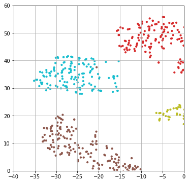
UMAPを実行
import umap
from scipy.sparse.csgraph import connected_components
# 公式GitHubには書いてあるのですが、↑を書かないとエラーが出てしまいます。
# sec: 実行

res_umap = umap.UMAP().fit_transform(digits.data)
print(res_umap.shape)
(1797, 2)
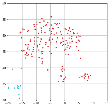
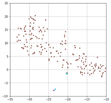
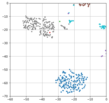
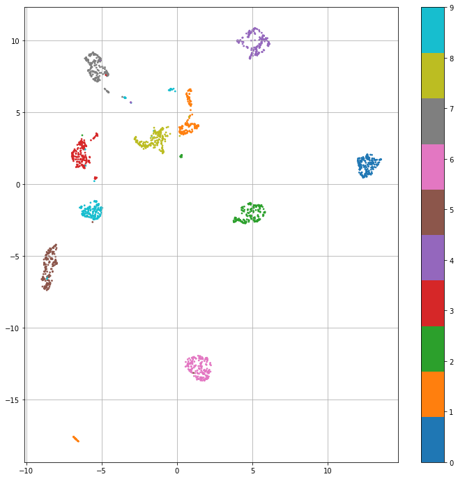
# sec: 結果の描画
import matplotlib.cm as cm
plt.figure(figsize=(12, 12))
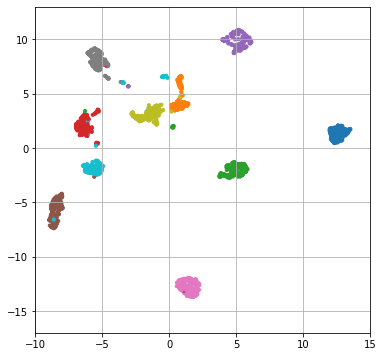
plt.scatter(res_umap[:,0], res_umap[:,1], s=3, c=digits.target, cmap=cm.tab10)
plt.colorbar()
plt.grid()
plt.show()
結果のグループを調べる
# sec: 結果を保存 毎回実行で変わる為

import pickle
with open("./results/2003 t-SNE/res-umap-1.pickle", 'wb') as file:
    pickle.dump(res_umap, file)
# sec: 結果を読み込み 前回の続きから

import pickle
with open("./results/2003 t-SNE/res-umap-1.pickle", 'rb') as file:
    res_umap = pickle.load(file)
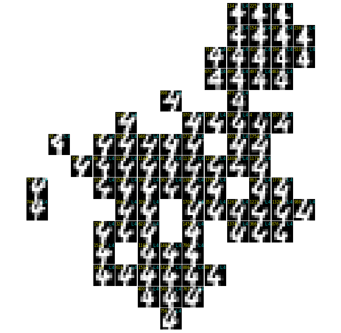
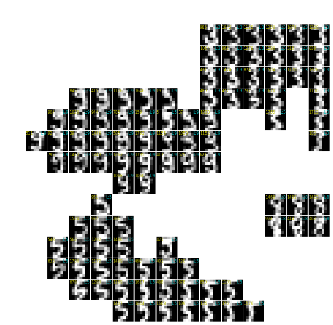
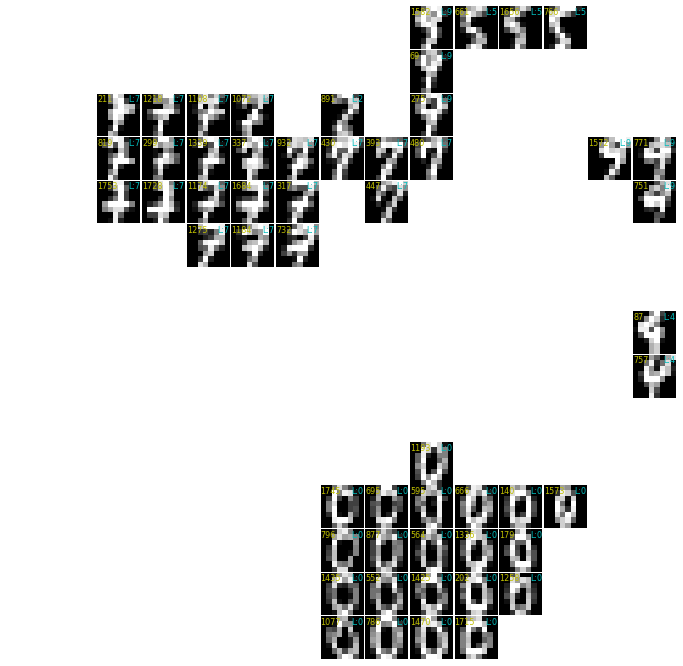
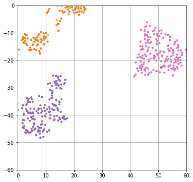
各数字の集団の分布状況を描画
# sec: 各場所の数字の分布状況を描画
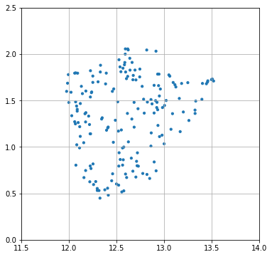
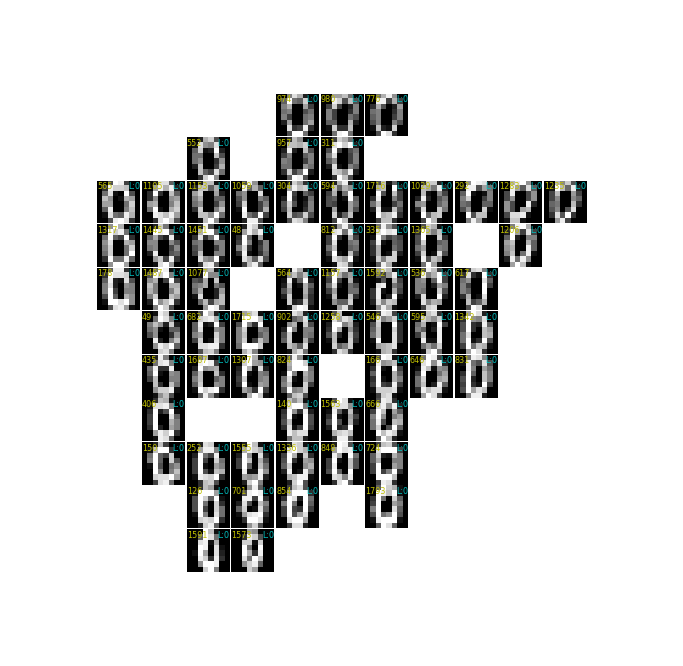
draw_digits_at_tsne(res_umap, 11.5, 14, 0, 2.5) # 0周り
draw_digits_at_tsne(res_umap, 0, 1.5, 3, 7) # 1周り
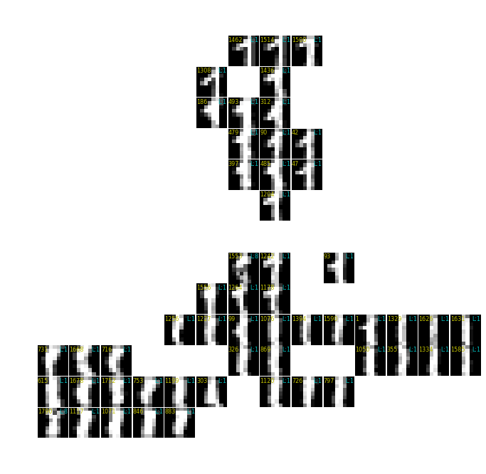
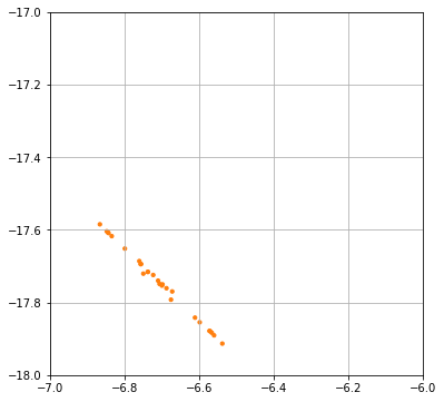
draw_digits_at_tsne(res_umap, -7, -6, -18, -17) # 1周り
draw_digits_at_tsne(res_umap, 3, 6.5, -3, -1) # 2周り
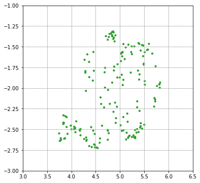
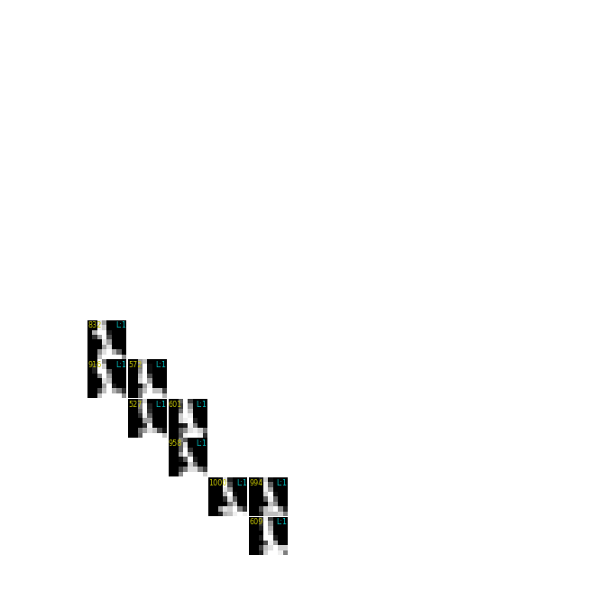
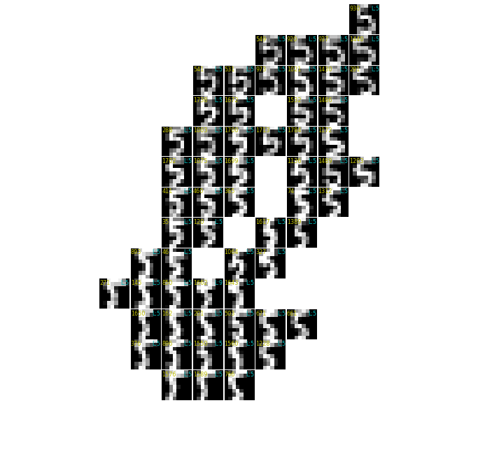
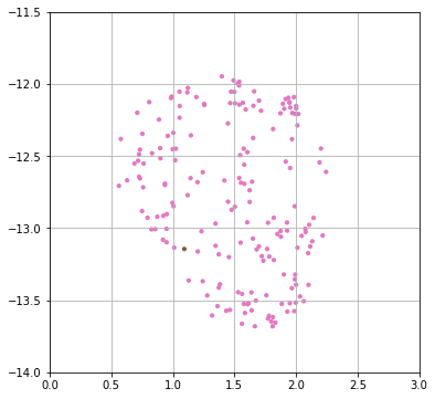
draw_digits_at_tsne(res_umap, -7.5, -5, 0, 4) # 3周り
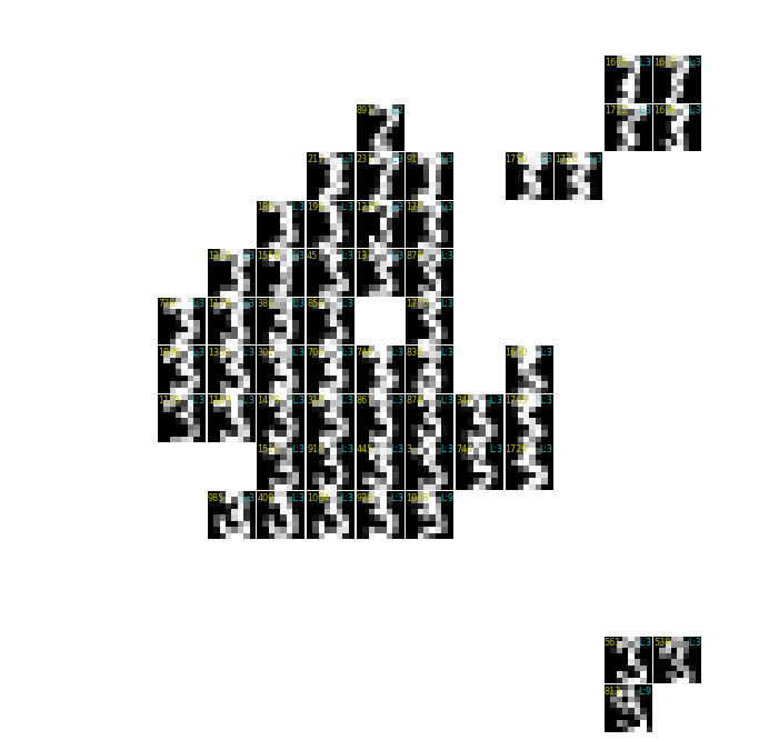
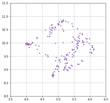
draw_digits_at_tsne(res_umap, 3.5, 6.5, 8, 11.5) # 4周り
draw_digits_at_tsne(res_umap, -9.5, -7.5, -8, -4) # 5周り
draw_digits_at_tsne(res_umap, 0, 3, -14, -11.5) # 6周り
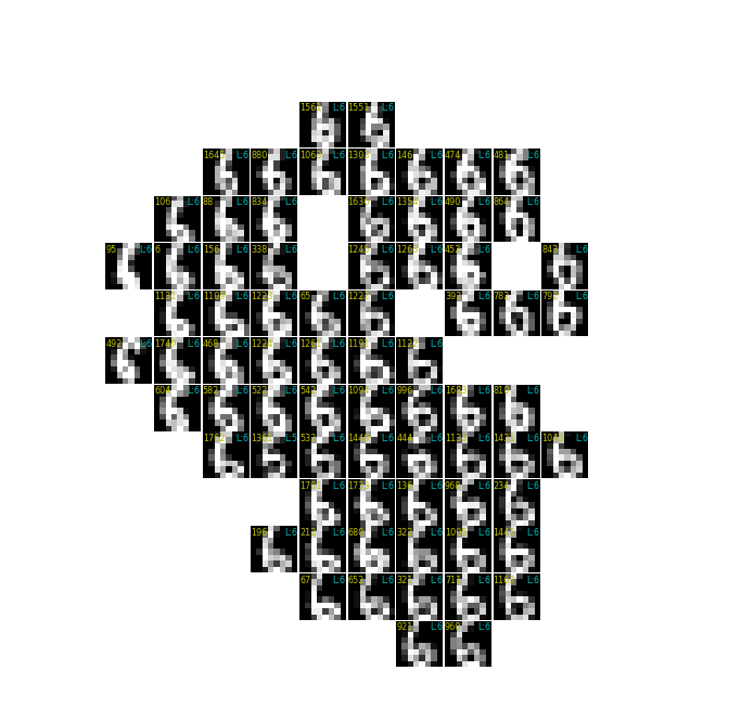
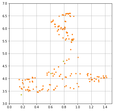
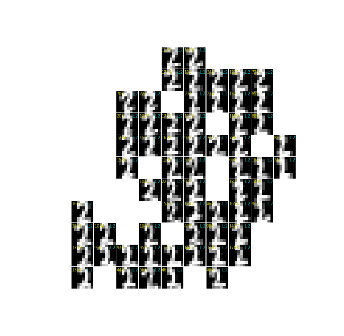
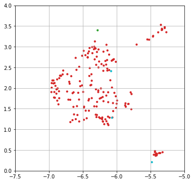
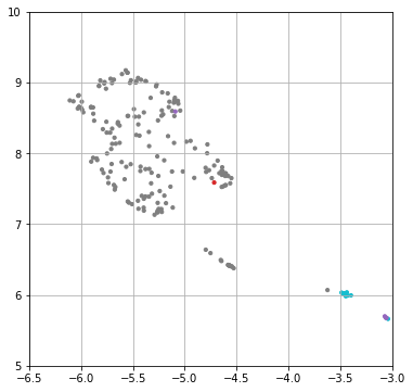
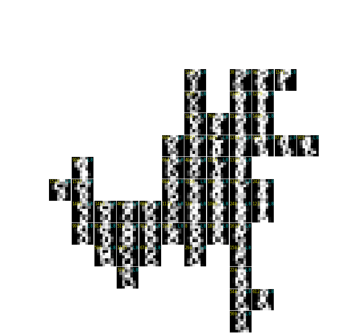
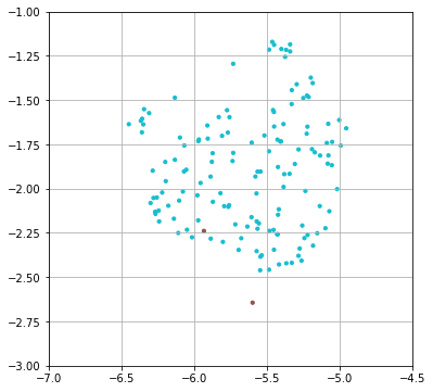
draw_digits_at_tsne(res_umap, -6.5, -3, 5, 10) # 7周り
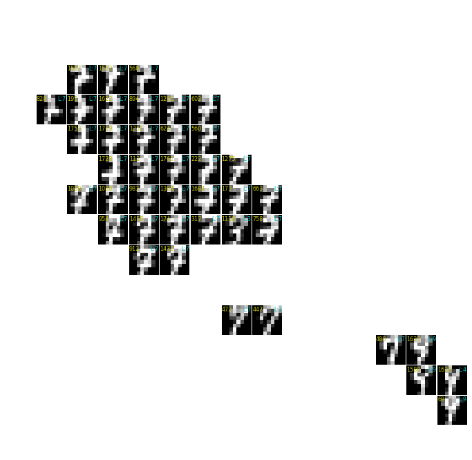
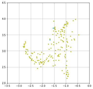
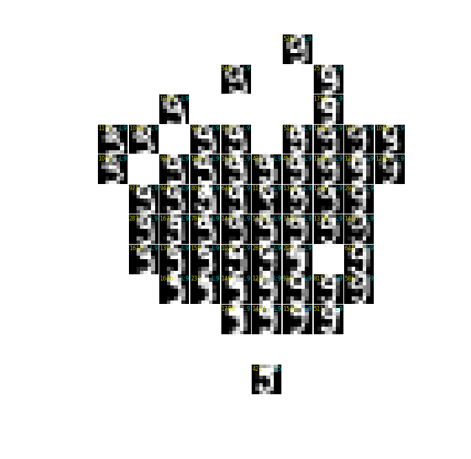
draw_digits_at_tsne(res_umap, -3.5, 0, 2, 4.5) # 8周り
draw_digits_at_tsne(res_umap, -7, -4.5, -3, -1) # 9周り
全体の分布状況を描画
draw_digits_at_tsne(res_umap, -10, 15, -17, 13, n_grid=(50, 50), annosize=None)