Rで厳密制約サポートベクトルマシン

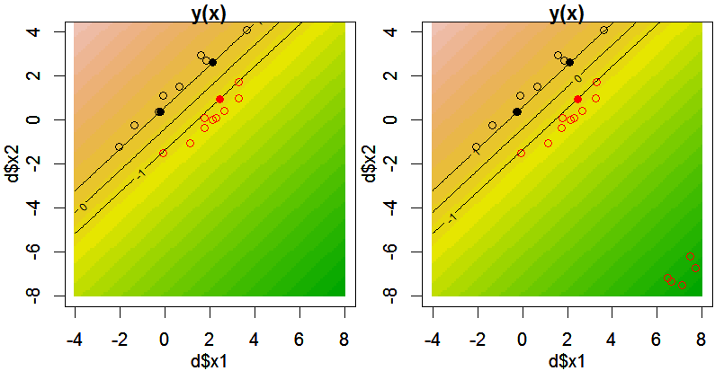
PRML 7.1に記載の、線形分離可能なデータを分類するサポートベクトルマシンを構成し、推定値、およびサポートベクトルを図示します。なお、カーネル関数は用いておらず、線形カーネル相当となります。二次計画法には、kernlabパッケージのipopを用いています。

library(MASS)
library(kernlab)
frame()
set.seed(0)
par(mfcol=c(1, 2))
par(mar=c(3, 3, 1, 0.1))
par(mgp=c(2, 1, 0))
xrange <- c(-4, 8)
yrange <- c(-8, 4)
x1 <- seq(xrange[1], xrange[2], .1)
x2 <- seq(yrange[1], yrange[2], .1)
x <- mvrnorm(10, c(0,1), matrix(c(2, 1.9, 1.9, 2), 2))
d1 <- as.data.frame(cbind(x, 1, 1))
x <- mvrnorm(10, c(2,0), matrix(c(2, 1.9, 1.9, 2), 2))
d1 <- rbind(d1, as.data.frame(cbind(x, 2, -1)))
x <- mvrnorm(5, c(7,-7), matrix(c(.2, 0, 0, .2), 2))
d2 <- rbind(d1, as.data.frame(cbind(x, 2, -1)))
d3 <- as.data.frame(rbind(cbind(1, 1, 1, 1), cbind(0, 1, 2, -1)))
names(d1) <- c("x1","x2","class","t")
names(d2) <- c("x1","x2","class","t")
names(d3) <- c("x1","x2","class","t")

doplot <- function(d) {
    N <- nrow(d)

    # quadratic programming
    cc <- matrix(rep(-1, N))
    hmat <- cbind(d$t * d$x1, d$t * d$x2)
    hmat <- hmat %*% t(hmat)
    ll <- matrix(rep(0, N))
    uu <- matrix(rep(1.0e+8, N)) # don't need the upper bound, though...
    bb <- 0
    rr <- 0
    amat <- matrix(d$t, nrow=1, ncol=N)
    sv <- ipop(cc, hmat, amat, bb, ll, uu, rr)
    a <- primal(sv)

    # non-support vectors
    a[a < 1.0e-5] <- 0

    # derive b
    bs <- c()
    for (n in 1:N) {
        if (a[n] != 0) {
            bs <- c(bs, d$t[n] - rowSums(a * d$t * (cbind(d$x1[n], d$x2[n]) %*% t(cbind(d$x1, d$x2)))))
        }
    }
    b <- mean(bs)

    # plot estimates
    estimate <- function(x1, x2) {
        result <- 0
        for (n in 1:N) {
            if (a[n] != 0) {
                result <- result + a[n] * d$t[n] * (cbind(x1, x2) %*% t(cbind(d$x1[n], d$x2[n])))
            }
        }
        result <- result + b
    }
    y1 <- outer(x1, x2, estimate)
    plot(d$x1, d$x2, col=d$class, type="n", xlim=xrange, ylim=yrange)
    image(x1, x2, y1, xlim=xrange, ylim=yrange, col=terrain.colors(32), add=T)
    contour(x1, x2, y1, xlim=xrange, ylim=yrange, levels=c(-1, 0, 1), add=T)
    par(new=T)
    plot(d$x1, d$x2, pch=ifelse(a == 0, 1, 16), col=d$class, xlim=xrange, ylim=yrange)
    title("y(x)")
}

doplot(d1)
doplot(d2)