RでEMアルゴリズムによる混合ベルヌーイモデル最尤推定

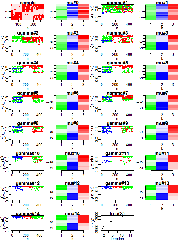
PRML 9.3.3に記載の通り、EMアルゴリズムによって混合ベルヌーイモデルの最尤推定が行われる過程と、対数尤度関数の収束の様子を示します。

10次元2値サンプルを、3種のベルヌーイ分布に従って、150サンプルずつ順に生成し、それらのサンプルに対する対数尤度を最大化します。EMステップ毎に、各サンプルについて、その混合要素のうち、最大の負担率γ(z_nk)の値を、その混合要素を示す色で記します。また、各混合要素について、ベルヌーイ分布のパラメータμkの値を示します。

また、MNISTの手書き数字文字データから生成した784(=28x28)次元2値データについて、数字2,3,4を各150サンプルずつ利用し、それらのサンプルに対する対数尤度を最大化します。

frame()
set.seed(0)
par(mfrow=c(8, 4))
par(mar=c(2.3, 2.5, 1, 0.1))
par(mgp=c(1.3, .5, 0))
MNIST <- F  # to load the MNIST handwritten digits
K <- 3
N <- 450

rbern <- function(mu) {
    ifelse(runif(length(mu)) < mu, 1, 0)
}
logdbern <- function(x, mu) {
    sum(log(mu ^ x * (1 - mu) ^ (1 - x)))
}
logsumexp <- function (x) {
  m <- max(x)
  m + log(sum(exp(x - m)))
}

if (MNIST) {
    # the following code is taken from https://gist.github.com/brendano/39760
    load_mnist <- function() {
      load_image_file <- function(filename) {
        ret = list()
        f = file(filename,'rb')
        readBin(f,'integer',n=1,size=4,endian='big')
        ret$n = readBin(f,'integer',n=1,size=4,endian='big')
        nrow = readBin(f,'integer',n=1,size=4,endian='big')
        ncol = readBin(f,'integer',n=1,size=4,endian='big')
        x = readBin(f,'integer',n=ret$n*nrow*ncol,size=1,signed=F)
        ret$x = matrix(x, ncol=nrow*ncol, byrow=T)
        close(f)
        ret
      }
      load_label_file <- function(filename) {
        f = file(filename,'rb')
        readBin(f,'integer',n=1,size=4,endian='big')
        n = readBin(f,'integer',n=1,size=4,endian='big')
        y = readBin(f,'integer',n=n,size=1,signed=F)
        close(f)
        y
      }
      train <<- load_image_file('mnist/train-images-idx3-ubyte')
      train$y <<- load_label_file('mnist/train-labels-idx1-ubyte')
    }
    # the data is available at http://yann.lecun.com/exdb/mnist/
    # extract the files in the "mnist" directory
    setwd("C:/Users/Public/Documents")
    load_mnist()
    x <- floor(rbind(
        train$x[train$y == 2, ][1:(N / 3), ],  
        train$x[train$y == 3, ][1:(N / 3), ],  
        train$x[train$y == 4, ][1:(N / 3), ]) / 128)
    D <- ncol(x)
} else {
    PHI <- 0.9
    PLO <- 0.1
    muorg <- matrix(c(
        PHI, PHI, PHI, PHI, PHI, PLO, PLO, PLO, PLO, PLO, 
        PLO, PLO, PLO, PLO, PLO, PHI, PHI, PHI, PHI, PHI, 
        PHI, PHI, PHI, PLO, PLO, PLO, PLO, PHI, PHI, PHI
        ), 3, byrow=T)
    z <- rep(1:3, each=N/3)
    x <- rbern(muorg[z, ])
    D <- 10
}
image(1:N, 1:D, x, xlab="n", ylab="i", breaks=seq(0, 1, 0.1), 
    col=hsv(0, seq(0.1, 1, 0.1), 1))
title("sample")

mu <- matrix(runif(D * K), K, byrow=T)
pz <- rep(1 / K, K)
gamma <- matrix(NA, nrow=N, ncol=K)
likelihood <- numeric()

iteration <- 0
repeat {
    cat("mu\n");print(mu)
    cat("pi\n");print(pz)

    if (!is.na(gamma[1, 1])) {
        plot(apply(gamma, 1, max), col=hsv(apply(gamma, 1, which.max) / K, 1, 1), 
            ylim=c(0, 1.05), pch=20, xlab="n", ylab=expression(gamma(z_nk)))
        title(paste0("gamma#", iteration))
    }

    if (MNIST) {
        image(1:28, 1:(28*K), matrix(as.vector(t(mu + rep(0:(K-1), D) + 1.0E-8)), nrow=28)[, (28*K):1], 
            axes=F, xlab="i", ylab="k", 
            breaks=seq(0, K, 0.1), 
            col=outer(seq(0.1, 1, 0.1), (1:K)/K, function(x1, x2) hsv(x2, x1, 1)))
        axis(1)
        axis(2, at=0:(K-1) * 28 + 14, labels=1:K)
    } else {
        image(1:K, 1:D, mu + rep(0:(K-1), D) + 1.0E-8, 
            axes=F, xlab="k", ylab="i",
            breaks=seq(0, K, 0.1), 
            col=outer(seq(0.1, 1, 0.1), (1:K)/K, function(x1, x2) hsv(x2, x1, 1)))
        axis(1, at=1:K)
        axis(2)
    }
    title(paste0("mu#", iteration))

    # E step
    for (n in 1:N) {
        pzx <- sapply(
            1:K, 
            function(k) log(pz[k]) + logdbern(x[n, ], mu[k, ])
            )
        pzx <- pzx - max(pzx)
        gamma[n, ] <- exp(pzx) / sum(exp(pzx))
    }

    # M step
    nk <- colSums(gamma)
    for (k in 1:K) {
        mu[k, ] <- colSums(x * gamma[, k]) / nk[k]
        pz[k] <- nk[k] / N
    }

    # likelihood
    likelihood <- c(likelihood, sum(sapply(1:N, function(n)
            logsumexp(sapply(
                1:K, 
                function(k)
                    log(pz[k]) + logdbern(x[n, ], mu[k, ])
                ))
            )))

    if (length(likelihood) > 1 
        && likelihood[length(likelihood)] - likelihood[length(likelihood) - 1] < 1.0E-2) {
        break
    }
    iteration <- iteration + 1
}

plot(likelihood, type="l", xlab="iteration", ylab="ln p(X)")
title("ln p(X)")