RでIRLSによるロジスティック回帰モデル最尤推定

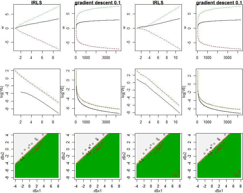
PRML4.3.3の通り、IRLS（反復再重み付け最小二乗法）によりロジスティック回帰モデルのパラメータwの最尤推定を行い、各xにおけるクラスの事後確率を求め、図4.4と同様に図示します。IRLSの過程でのwおよび▽E(w)の変化も図示します。また、勾配降下法で解いた場合についても図示します。

library(MASS)
frame()
set.seed(0)
par(mfcol=c(3, 4))
par(mar=c(3, 3, 1, 0.1))
par(mgp=c(2, 1, 0))
xrange <- c(-4, 8)
yrange <- c(-8, 4)
x1 <- seq(xrange[1], xrange[2], .1)
x2 <- seq(yrange[1], xrange[2], .1)
x <- mvrnorm(10, c(0,1), matrix(c(2, 1.9, 1.9, 2), 2))
d1 <- as.data.frame(cbind(x, 1, 1))
x <- mvrnorm(10, c(2,0), matrix(c(2, 1.9, 1.9, 2), 2))
d1 <- rbind(d1, as.data.frame(cbind(x, 2, 0)))
x <- mvrnorm(5, c(7,-7), matrix(c(.2, 0, 0, .2), 2))
d2 <- rbind(d1, as.data.frame(cbind(x, 2, 0)))
names(d1) <- c("x1","x2","class","t")
names(d2) <- c("x1","x2","class","t")

logistic <- function(x) {
        1 / (1 + exp(-x))
}
base <- function(x1, x2) {
        (cbind(1, x1, x2))   # w0をバイアス項とするためφ0=1
}
doplot <- function(d, irls) {
        eta <- 0.1
        w = c(0, 0, 0)
        weights <- w
        phi <- base(d$x1, d$x2)
        grads <- c()
        repeat {
                y <- t(logistic(t(w) %*% t(phi)))
                g <- t(phi) %*% (y - d$t)
                grads <- rbind(grads, t(g))
                if (sum(g^2) < 1.0e-5) break
                if (irls) {
                        rn <- as.vector(y * (1 - y))
                        r <- diag(rn)
                        hessian <- t(phi) %*% r %*% phi
                        #rinv <- diag(1 / rn)
                        #z <- phi %*% w - rinv %*% (y - d$t)
                        #w <- solve(hessian) %*% t(phi) %*% r %*% z
                        diff <- solve(hessian) %*% t(phi) %*% (y - d$t)
                        w <- w - diff
                } else {
                        diff <- 0.1 * g
                        w <- w - diff
                }
                weights = rbind(weights, t(w))
        }
        matplot(weights, type="l", ylab="w", main=ifelse(irls, "IRLS", paste("gradient descent", eta)))
        matplot(log(abs(grads)), type="l", ylab=expression(paste("log", group("|", paste(nabla, "E"), "|"))))
        estimate <- function(x1, x2){
                logistic(t(w) %*% t(base(x1, x2)))
        }
        y1 <- outer(x1, x2, estimate)
        contour(x1, x2, y1, xlim=xrange, ylim=yrange, levels=c(0.5))
        image(x1, x2, y1, xlim=xrange, ylim=yrange, zlim=c(0,1), col=terrain.colors(32), add=T)
        contour(x1, x2, y1, xlim=xrange, ylim=yrange, levels=c(0.5), add=T)
        par(new=T)
        plot(d$x1, d$x2, col=d$class, xlim=xrange, ylim=yrange)
}

doplot(d1, T)
doplot(d1, F)
doplot(d2, T)
doplot(d2, F)