Rで線形基底関数モデルの予測分布

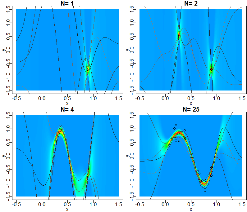
PRML図3.8と同様に、ガウス基底を基底関数とする線形基底関数モデルにおいて、サンプルから求めた重みの事後分布から、予測値の予測分布を求め、サンプル点とともに図示します。また、図3.9と同様に、重みの事後分布から生成した関数の例を図示します。

library(mvtnorm)
frame()
set.seed(0)
par(mfrow=c(2, 2))
par(mar=c(2, 2, 1, 0.1))
par(mgp=c(1, 0.2, 0))
xrange <- c(-0.5, 1.5)
yrange <- c(-1.5, 1.5)
x1 <- seq(xrange[1], xrange[2], .01)
x2 <- seq(yrange[1], yrange[2], .01)
colors <- rainbow(450)[256:1]
M <- 10
N <- 25

base <- function(m, x) {
#	r <- x^m						#多項式基底の場合
	r <- exp(-(x-(m-1)/(M-2))^2/(2*0.2^2))	#ガウス基底の場合
	r[m == 0]<-1					# w0をバイアス項とするためφ0=1
	r
}
makePhi<-function(M, x) {
	A <- matrix(nrow=length(x), ncol=M)
	for (i in 1:length(x)) {
		for (j in 0:(M-1)) {
			A[i, 1+j] <- base(j, x[i])
		}
	}
	A
}
x <- runif(N, 0, 1)
y <- rnorm(N, sin(2 * pi * x), 0.2)

alpha <- 0.1
beta <- (1 / 0.2) ^ 2

# prior probability distribution
s0inv <- alpha * diag(1, M)
m0 <- rep(0, M)
cat("s0");print(solve(s0inv))
cat("m0");print(m0)
 
for (n in c(1, 2, 4, 25)) {
	# derive the posterior
	phi <- makePhi(M, x[1:n])
	sninv <- s0inv + beta * t(phi) %*% phi
	sn <- solve(sninv)
	mn <- sn %*% (s0inv %*% m0 + beta * t(phi) %*% y[1:n])
	cat("sn");print(sn)
	cat("mn");print(mn)
	
	plot(x[1:n], y[1:n], xlim=xrange, ylim=yrange, xlab="x", ylab="y")
	title(paste("N=", n))
	
	# derive the predictive distribution
	phin <- t(makePhi(M, x1))
	u <- t(mn) %*% phin
	s <- 1 / beta + diag(t(phin) %*% sn %*% phin)
	predictive <- function(x, y) {
			dnorm(y, u[x], s[x])
	}
	image(x1, x2, outer(1:length(x1), x2, predictive), xlim=xrange, ylim=yrange, col=colors, xlab="", ylab="", axes=F, add=T)
	
	# plot example regressions
	for (i in 1:5) {
			w <- rmvnorm(1, mn, sn)
			estimate<-function(x){
					(w %*% t(makePhi(M, x)))  # (w[1]+w[2]*base(1,x)+w[3]*base(2,x)...)
			}
			par(new=T)
			curve(estimate, type="l", xlim=xrange, ylim=yrange, col=gray(i/10), xlab="", ylab="", axes=F)
	}
	
	# plot the samples
	par(new=T)
	plot(x[1:n], y[1:n], xlim=xrange, ylim=yrange, xlab="", ylab="", axes=F)
}