お天気データで異常検知

勉強がてら、気象庁が公開している気象データで異常検知をしてみました（異常気象とは言っていない）。

コード全文は以下です。
https://github.com/shibuiwilliam/weather_outlier

動機

自己学習のため　＆　2/14にやってた異常検知ナイトが面白かったためです。

使ったデータ

以下で取得した気象庁が公開している気象データを使いました。
Japan Meteorogical Agency
東京地方を選択し、日別で30年分を取得しています。

詳しくは以下です。

地域：東京>東京
期間：1987/01/01-2017/12/31
単位：日別
項目：平均気温、最高気温、最低気温、雨量、日照時間、最深積雪、平均風速、最高風速、最高風速の向き

気象庁が公開している項目は上記よりも多種多様にあります。
上記を選んだのは、1度のダウンロードで1年分を取得できるように調節した結果、上記がちょうど良かったためです。

データは分析にあたり、月間でまとめなおしています。
全データをまとめて異常検知してもよかったのですが、季節性を考慮して月ごとに異常検知にかけるようにしました。

使った異常検知

scikit-learnが用意している教師なし学習系のライブラリを使いました。
具体的には以下です。

OneClassSvm
KernelDensity
LocalOutlierFactor
GaussianMixture
IsolationForest
EllipticEnvelope

手順

以下の手順でやってみました。

データ収集
データ整備
異常検知
結果表示

データ収集

Japan Meteorogical Agencyから手動でデータをダウンロードしました。
ダウンロードしたデータはCSVになります。
1回にダウンロードできる容量は制限されているため、1年＝1ダウンロードで30年分をダウンロードし、そのあとで1ファイルに時系列で結合しました。

また、項目名は日本語で取得されるのですが、利便性のために英語に変更します。

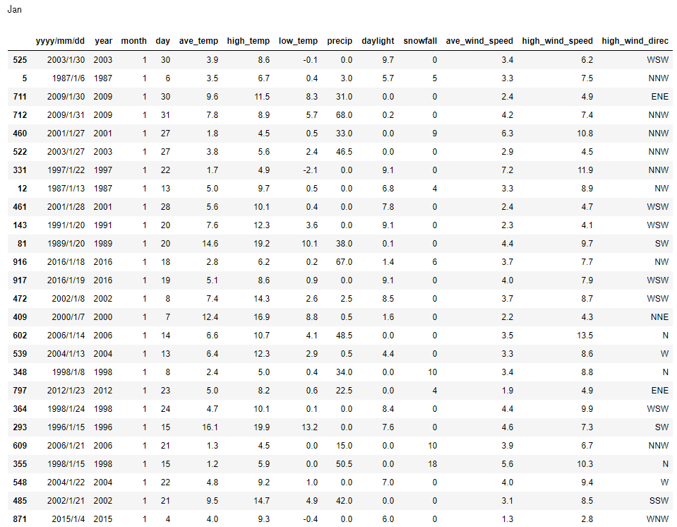
データは以下のようなものになります。

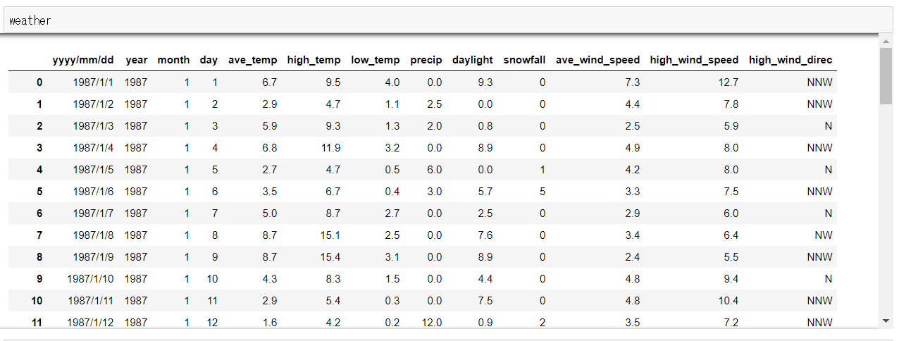
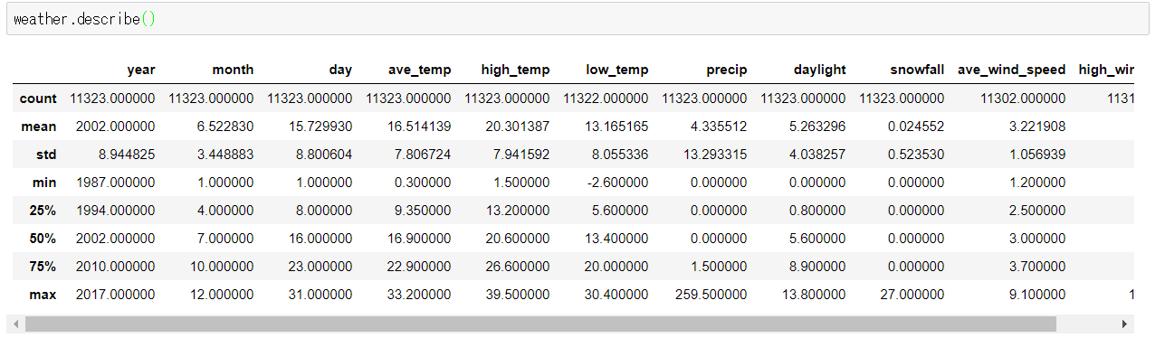
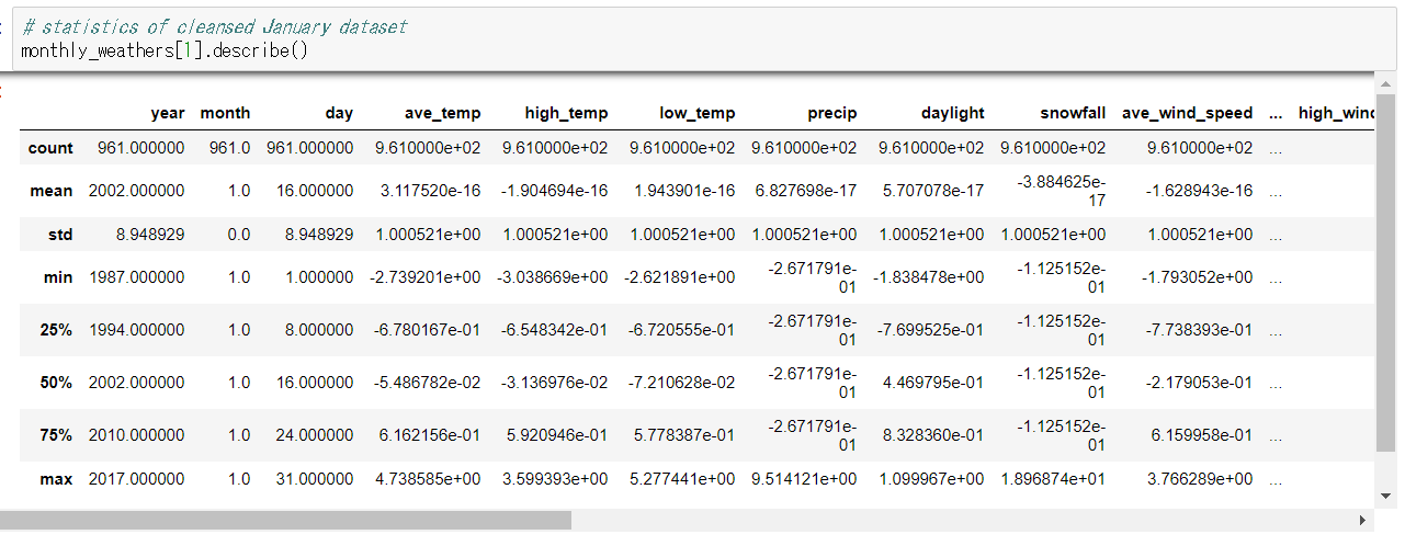
統計をとるとこんな感じです。

ここでデータを月ごとに分けます。


# dividing the original dataset to monthly datasets
orig_monthly_weathers = {}
for i in range(1,13,1):
    orig_monthly_weathers[i] = weather.query("month=={0}".format(i))
    orig_monthly_weathers[i].reset_index(inplace=True, drop=True)

月ごとに分けたデータに対し、外れ値の有無を確認するため、ためしにボックスプロットを書いてみます。


r = ['ave_temp', 'high_temp', 'low_temp', 'precip','daylight', 'snowfall', 'ave_wind_speed', 'high_wind_speed']
for i in range(1,13,1):
    fig = plt.figure()
    ax = fig.add_subplot(111)
    ax.boxplot(np.array(orig_monthly_weathers[i][r]))
    ax.set_xticklabels(r)
    plt.title(months[i-1])
    plt.grid()
    plt.show()

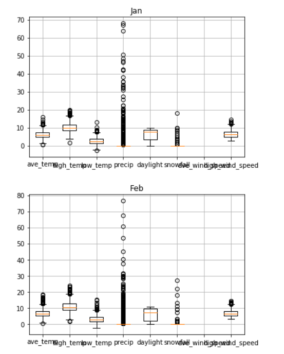
この時点で雨量や積雪、風速でところどころ外れ値が存在することがわかります。

データ整備

元データは意外とキレイで欠損値も少ないのですが（さすが気象庁）、ところどころ分析しやすいように修正します。
データ整備には以下を実施しました。

最高風速の風向きが名義尺度になっているので、これをダミー変数をとって数値（0，1）に変換します。
欠損値を月間平均値で埋めます。
連続値データを標準化します（平均0、標準偏差1）。

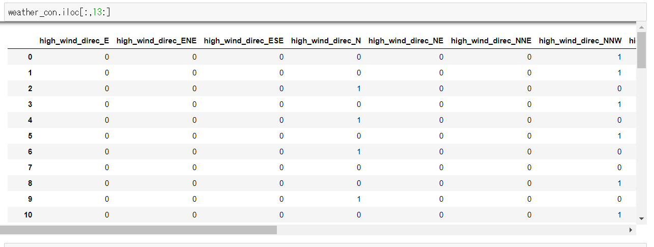
ダミー変数

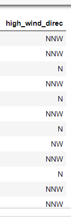
風向きは東西南北（EWSN）で表されているので、これをダミー変数にします。
ダミー変数にすることで、風向きが東北の場合はNEカラムが1、他のカラムは0という形式に変換することができます。
こうすることで名義尺度を数値として扱うことができるようになります。

# get dummy columns for high_wind_direc to tranpose nominal scale to numerical scale
high_wind_dummies = pd.get_dummies(weather[["high_wind_direc"]])
weather_con = pd.merge(weather, high_wind_dummies, left_index=True, right_index=True)

↓↓↓

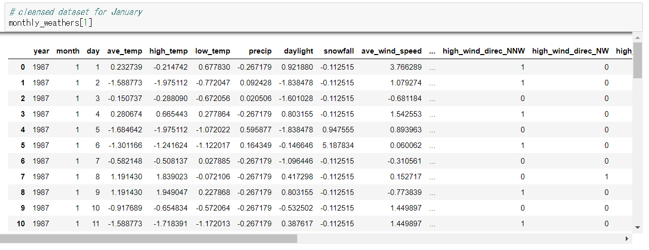
欠損値補完と標準化

欠損値（Null値）を月間の平均値で補完します。
また、数値データのバラツキをなくすため、標準化して値を平均0、標準偏差1の間に集約します。

# imputation
imp = preprocessing.Imputer(missing_values='NaN', strategy='mean', axis=0, copy=True)
# standard scaler
ss = preprocessing.StandardScaler()
ss_columns = columns_to_use[3:11]

for m,w in monthly_weathers.items():
    # finding if there's null value
    has_null = [c for c in columns_to_use if len(w[w[c].isnull()]) > 0]
    if has_null != []:
        # impute null values
        w_with_nan = w[has_null]
        imp_w = imp.fit_transform(w_with_nan).T
        for i in range(len(has_null)):
            # replace columns with null to the imputed
            w[has_null[i]] = imp_w[i]
            if len(w[w[has_null[i]].isnull()]) > 0:
                print(has_null[i], len(w[w[has_null[i]].isnull()]))
    # standard scaler
    w[ss_columns] = pd.DataFrame(ss.fit_transform(w[ss_columns]), columns=ss_columns)

ここまでで1月のデータは以下のように変換されました。

異常検知

データが整備されたので、異常検知してみます。
この異常検知では、毎月のデータに異常検知をかけていき、データが他から外れている日を検知します。

異常検知は以下を適用して実施します。

OneClassSvm
KernelDensity
LocalOutlierFactor
GaussianMixture
IsolationForest
EllipticEnvelope

OneClassSvm、LocalOutlierFactor、IsolationForest、EllipticEnvelopeはoutliers_fractionを設定することで異常と判定する割合を指定することができます。
今回は1％を異常と判定するようにします。

KernelDensityとGaussianMixtureにはそのような設定値はありません。
自分で閾値を設定してその外れ値を異常とします。
今回はKernelDensityとGaussianMixtureも同様に1％程度を以上と判定するよう、パラメータを調整しました。

outliers_fraction = 0.01
rng = np.random.RandomState(123)
anomaly_list = ["ellipticEnvelope", "kernelDensity", "gaussianMixture", 
                "localOutlierFactor", "isolationForest", "oneClassSVM"]

def ellipticEnvelope(inputs):
    """
    inputs: dataset
    returns:
        score_pred: evaluated scores on each day
        outlier_rows: rows evaluated as 1% outliers
    """
    clf = EllipticEnvelope(contamination=outliers_fraction)
    clf.fit(inputs)
    score_pred = clf.decision_function(inputs)
    pred = clf.predict(inputs)
    outlier_rows = [i for i in range(len(pred)) if pred[i]==-1]
    return score_pred,outlier_rows

def kernelDensity(inputs):
    """
    inputs: dataset
    returns:
        score_pred: evaluated scores on each day
        outlier_rows: rows evaluated as outliers
            On kernel density estimator, I defined rows with score 
            lower than 1.125 times the average as outliers
    """
    clf = KernelDensity(bandwidth=1, kernel="gaussian")
    clf.fit(inputs)
    score_pred = clf.score_samples(inputs)
    pred = np.where(score_pred <= np.average(score_pred)*1.125, -1, 1)
    outlier_rows = [i for i in range(len(pred)) if pred[i]==-1]
    return score_pred,outlier_rows

def gaussianMixture(inputs):
    """
    inputs: dataset
    returns:
        score_pred: evaluated scores on each day
        outlier_rows: rows evaluated as outliers
            On kernel density estimator, I defined rows with score 
            lower than 0.7 times the average as outliers
    """
    clf = GaussianMixture(n_components=5, covariance_type="full")
    clf.fit(inputs)
    score_pred = clf.score_samples(inputs)
    pred = np.where(score_pred <= np.average(score_pred)*0.7, -1, 1)
    outlier_rows = [i for i in range(len(pred)) if pred[i]==-1]
    return score_pred,outlier_rows

def localOutlierFactor(inputs):
    """
    inputs: dataset
    returns:
        score_pred: evaluated scores on each day
        outlier_rows: rows evaluated as 1% outliers
    """
    clf = LocalOutlierFactor(n_neighbors=20, contamination=outliers_fraction)
    clf.fit(inputs)
    score_pred = clf._decision_function(inputs)
    pred = clf._predict(inputs)
    outlier_rows = [i for i in range(len(pred)) if pred[i]==-1]
    return score_pred,outlier_rows

def isolationForest(inputs):
    """
    inputs: dataset
    returns:
        score_pred: evaluated scores on each day
        outlier_rows: rows evaluated as 1% outliers
    """
    clf = IsolationForest(contamination=outliers_fraction,
                          max_samples="auto",
                          random_state=rng,
                          n_estimators=100)
    clf.fit(inputs)
    score_pred = clf.decision_function(inputs)
    pred = clf.predict(inputs)
    outlier_rows = [i for i in range(len(pred)) if pred[i]==-1]
    return score_pred,outlier_rows

def oneClassSVM(inputs):
    """
    inputs: dataset
    returns:
        score_pred: evaluated scores on each day
        outlier_rows: rows evaluated as 1% outliers
    """
    clf = svm.OneClassSVM(nu=outliers_fraction,
                          kernel="rbf",
                          gamma=0.03)
    clf.fit(inputs)
    score_pred = clf.decision_function(inputs).T[0]
    pred = clf.predict(inputs)
    outlier_rows = [i for i in range(len(pred)) if pred[i]==-1]
    return score_pred,outlier_rows

# Running each outlier detection on each month
monthly_pred = {}
for m,w in monthly_weathers.items():
    monthly_pred[m] = {}
    # elliptic envelope
    s,o = ellipticEnvelope(w[columns_to_analyze])
    monthly_pred[m]["ellipticEnvelope"] = {"score_pred":s, "outlier_rows":o}
    # kernel density estimator
    s,o = kernelDensity(w[columns_to_analyze])
    monthly_pred[m]["kernelDensity"] = {"score_pred":s, "outlier_rows":o}
    # gaussian mixture
    s,o = gaussianMixture(w[columns_to_analyze])
    monthly_pred[m]["gaussianMixture"] = {"score_pred":s, "outlier_rows":o}
    # local outlier factor
    s,o = localOutlierFactor(w[columns_to_analyze])
    monthly_pred[m]["localOutlierFactor"] = {"score_pred":s, "outlier_rows":o}
    # isolation forest
    s,o = isolationForest(w[columns_to_analyze])
    monthly_pred[m]["isolationForest"] = {"score_pred":s, "outlier_rows":o}
    # one class svm
    s,o = oneClassSVM(w[columns_to_analyze])
    monthly_pred[m]["oneClassSVM"] = {"score_pred":s, "outlier_rows":o}

これで各異常検知判定を各月に適用し、異常と判定された日が取得できました。

結果表示

結果を集計します。
各異常検知アルゴリズムによって異常と判定している日数や日には違いがあります。
異常と判定された日数とバラツキを見るため、以下で図示します。

stats_columns = ["MONTH","DATASIZE","NORMALS","ANOMALIES","ANOMALY_RATE"]
outliers = {}
for m in months:
    outliers[m] = {}

# drawing scatter plots on each algorithm, with month on y-axis
for aa in anomaly_list:
    data_size = []
    oks = []
    ngs = []
    ng_rate = []
    for i in range(1,13,1):
        # gathering outlier and normal rows on each month
        p_ng = monthly_pred[i][aa]["outlier_rows"]
        p_ok = np.delete(np.arange(0,num_rows[i]), p_ng)
        p_ng_score = monthly_pred[i][aa]["score_pred"][p_ng]
        p_ok_score = monthly_pred[i][aa]["score_pred"][p_ok]

        data_size.append(num_rows[i])
        oks.append(len(p_ok))
        ngs.append(len(p_ng))
        ng_rate.append(round(100*len(p_ng)/num_rows[i], 2))

        for n in p_ng:
            outliers[months[i-1]][n] = 1 if n not in outliers[months[i-1]].keys() else outliers[months[i-1]][n]+1

        # scatter plot 
        plt.scatter(p_ok_score, np.zeros(len(p_ok_score))+i, c="blue")
        plt.scatter(p_ng_score, np.zeros(len(p_ng_score))+i, c="red")

    print(aa)
    stats = pd.DataFrame(np.array([months,data_size,oks,ngs,ng_rate]).T, columns=stats_columns)
    display(stats)

    plt.title(aa)
    plt.xlabel("predicted scores")
    plt.ylabel("months")
    plt.grid(True)
    plt.show()

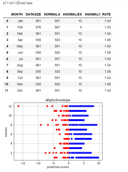
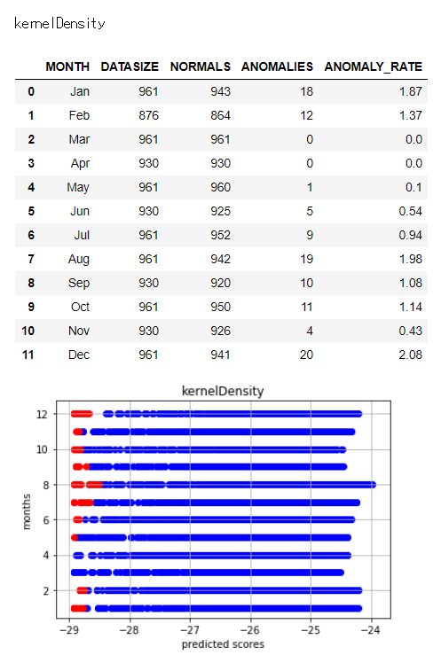
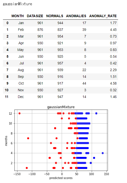
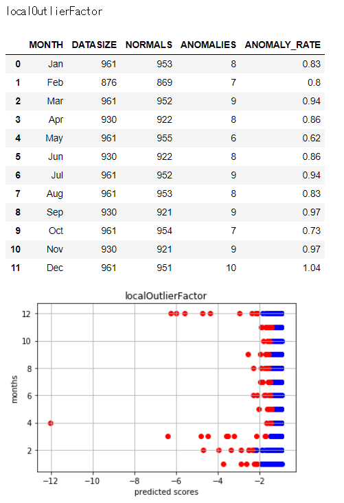
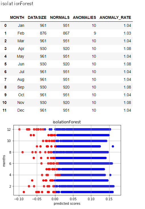
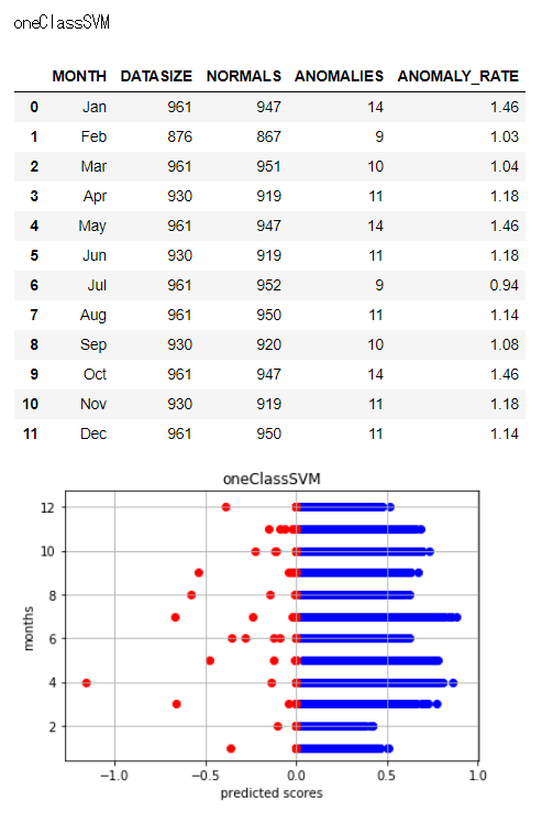
アルゴリズムによってバラツキ具合に差異があることがわかります。

上記で異常と判定された日にちを集計していますが、たとえば1月だけでも、異常と判定したアルゴリズムが1つだけのときもあれば、複数のアルゴリズムが異常と判定する日にちがあります（下記はキーを行番号、値を異常と判定したアルゴリズム数でとっています）。

'Jan':
 {5: 1,  12: 2,  54: 1,  81: 3,  84: 1,  108: 2,  143: 1,  245: 2,  293: 2,  331: 1,  348: 3,  349: 1,  355: 6,  364: 1,  409: 1,  417: 1,  421: 1,  460: 3,  461: 1,  472: 1,  485: 3,  491: 2,  522: 3,  524: 1,  525: 1,  539: 1,  548: 1,  573: 1,  602: 4,  609: 3,  711: 3,  712: 2,  797: 3,  819: 4,  871: 1,  901: 1,  916: 4,  917: 1,  924: 1,  944: 1,  949: 1}

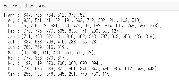
このうち、3以上のアルゴリズムが異常と判定した日にちを抽出します。

# pick up days detected by more than or equal to 3 algorithms
out_more_than_three = {}
for m,v in outliers.items():
    out_more_than_three[m] = []
    for k,n in v.items():
        if n >= 3:
            out_more_than_three[m].append(k)

# days detected by more than or equal to 3 algorithms
for i in range(1,13,1):
    print(months[i-1])
    display(orig_monthly_weathers[i].iloc[out_more_than_three[months[i-1]],:])

だいぶ見やすくなりました。

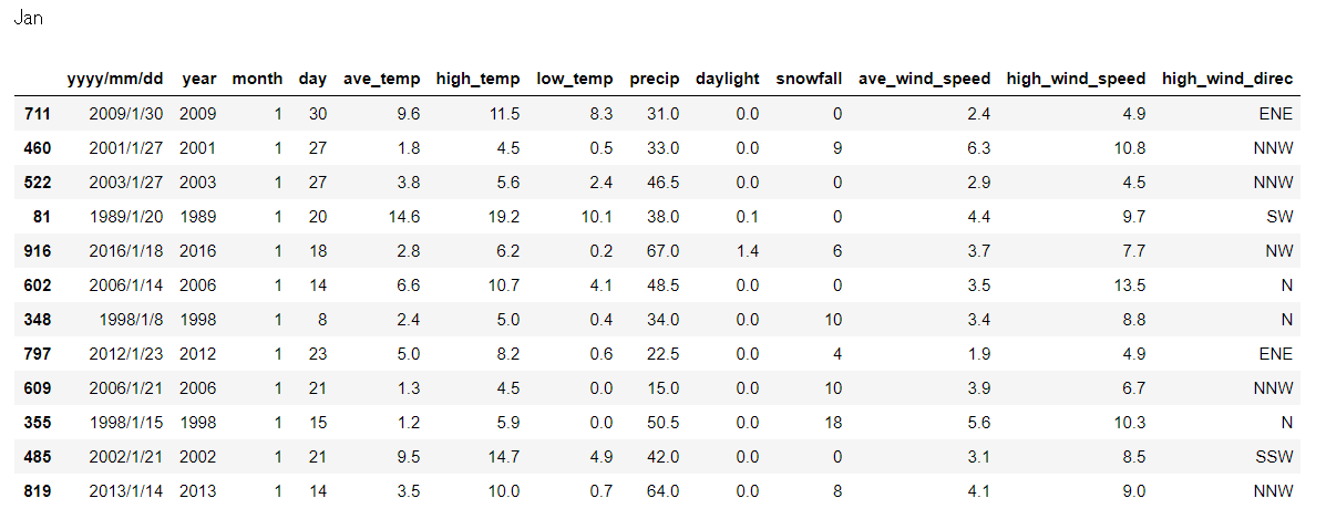
ちなみに1月で全6アルゴリズムが異常と判定しているのは1998/1/15でして、この日は関東大雪とのことでYouTubeにニュースが見つかりました。
https://www.youtube.com/watch?v=zeEcxqqPGFI

6アルゴリズムで異常判定されているのは以下があります。

1998/1/15 大雪
1993/8/27 大雨
2003/8/15 冷夏
1995/9/17 冷夏
1996/9/22 台風
2004/10/9 台風
2013/10/16 台風

参考リンク

http://scikit-learn.org/dev/auto_examples/plot_anomaly_comparison.html
http://scikit-learn.org/stable/auto_examples/covariance/plot_outlier_detection.html#sphx-glr-auto-examples-covariance-plot-outlier-detection-py
https://dllab.connpass.com/event/77248/
https://www.slideshare.net/KosukeNakago/dllab-20180214-88470902