PRML第14章 条件付き混合モデル Python実装

一つのモデルではデータの特徴を捉えられないので、複数のモデルを組み合わせたいというときに混合モデルを用います。今回はその中でも線形回帰モデルの混合を実装します。

線形回帰モデルの混合

入力$x$、出力$t$の普通の線形回帰モデルを確率的に表すと、

p(t|x,{\bf w},\beta) = \mathcal{N}(t|{\bf w}^\top\phi(x),\beta^{-1})

のようになります。ただし、$\phi(\cdot)$は特徴ベクトル、${\bf w}$は重み係数、$\beta$は精度パラメータとしています。　
混合線形回帰モデルでは混合係数$\pi_k$(ただし$\sum_k\pi_k=1$)を導入して、K個の線形回帰モデルを足し合わせて次のように表します。

p(t|x,{\bf W},\beta,\pi) = \sum_{k=1}^K\pi_k\mathcal{N}(t|{\bf w}_k^\top\phi(x),\beta^{-1})

例によって、学習データ$\{x_n,t_n\}_{n=1}^N$(以後${\bf t, x}$と表す)が与えられたときのパラメータ${\bf W},\pi,\beta$を最尤推定します。そのときの対数尤度関数は、

\ln p({\bf t}|{\bf x},{\bf W},\pi,\beta) = \sum_{n=1}^N\ln\left(\sum_{k=1}^K\pi_k\mathcal{N}(t_n|{\bf w}_k^\top\phi(x_n),\beta^{-1})\right)

となります。ここで、個々のデータがどのモデルから生成されたかを表す潜在変数$z_{nk}$を導入します。この潜在変数は0または1の値をとり、$z_{nk}=1$であればn番目のデータ点はk番目のモデルから生成されていることを表し、$1,\cdots,k-1,k+1,\cdots,K$については0となっている。
これで、完全データが与えられたときのパラメータについての対数尤度関数も書き下せます。

こうして、混合線形回帰モデルの最尤推定にEMアルゴリズムを使える形になりました。Eステップでは各データ点、各モデルについて$\mathbb{E}[z_{nk}]$を求め、Mステップでは完全データが与えられたときの対数尤度関数の潜在変数$z$についての事後分布による期待値をパラメータについて最大化します。

コード

import

今回は、いつものnumpyとmatplotlibに加えてpythonの標準ライブラリであるitertoolsもimportします。(本当はいらないけど)

import itertools
import matplotlib.pyplot as plt
import numpy as np

計画行列

行ベクトルがそれぞれの特徴ベクトルを表している計画行列をつくります。

class PolynomialFeatures(object):

    def __init__(self, degree=2):
        assert isinstance(degree, int)
        self.degree = degree

    def transform(self, x):
        if x.ndim == 1:
            x = x[:, None]
        x_t = x.transpose()
        features = [np.ones(len(x))]
        for degree in range(1, self.degree + 1):
            for items in itertools.combinations_with_replacement(x_t, degree):
                features.append(reduce(lambda x, y: x * y, items))
        return np.asarray(features).transpose()

条件付き混合モデル

一番のメイン部分である混合線形回帰モデルを行うためのコードです。

class ConditionalMixtureModel(object):

    def __init__(self, n_models=2):
        # モデルの個数を指定
        self.n_models = n_models

    # 最尤推定を行うメソッド
    def fit(self, X, t, n_iter=100):
        # 推定したいパラメータ（重み係数、混合係数、分散）の初期化
        coef = np.linalg.pinv(X).dot(t)
        self.coef = np.vstack((
            coef + np.random.normal(size=len(coef)),
            coef + np.random.normal(size=len(coef)))).T
        self.var = np.mean(np.square(X.dot(coef) - t))
        self.weight = np.ones(self.n_models) / self.n_models

        # EMステップを指定した回数だけ繰り返す
        for i in xrange(n_iter):
            # Eステップ 負担率E[z_nk]を各データ、各モデルごとに計算
            resp = self._expectation(X, t)

            # Mステップ パラメータについて最大化
            self._maximization(X, t, resp)

    # ガウス関数
    def _gauss(self, x, y):
        return np.exp(-(x - y) ** 2 / (2 * self.var))

    # Eステップ 負担率gamma_nk=E[z_nk]を計算
    def _expectation(self, X, t):
        # PRML式(14.37)
        responsibility = self.weight * self._gauss(X.dot(self.coef), t[:, None])
        responsibility /= np.sum(responsibility, axis=1, keepdims=True)
        return responsibility

    # Mステップ パラメータについて最大化
    def _maximization(self, X, t, resp):
        # PRML式(14.38) 混合係数の計算
        self.weight = np.mean(resp, axis=0)

        for m in xrange(self.n_models):
            # PRML式(14.42) 各モデルごとに係数を計算
            self.coef[:, m] = np.linalg.inv((X.T * resp[:, m]).dot(X)).dot(X.T * resp[:, m]).dot(t)

        # PRML式(14.44) 分散の計算
        self.var = np.mean(
            np.sum(resp * np.square(t[:, None] - X.dot(self.coef)), axis=1))

    def predict(self, X):
        return X.dot(self.coef)

学習データ

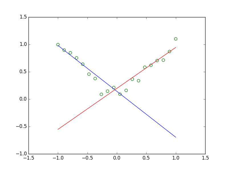
$y=|x|$に従う学習データを用意します。$x\ge0$と$x\le0$のそれぞれの範囲では一つの線形回帰モデルでフィッティングできますが、両方の範囲でフィッティングを行うには２つモデルを用意したほうが良いようにしました。

def create_toy_data(sample_size=20, std=0.1):
    x = np.linspace(-1, 1, sample_size)
    y = (x > 0.).astype(np.float) * 2 - 1
    y = x * y
    y += np.random.normal(scale=std, size=sample_size)
    return x, y

メイン関数

def main():
    # 学習データの作成
    x_train, y_train = create_toy_data()

    # 特徴ベクトルの定義（次数1）
    feature = PolynomialFeatures(degree=1)

    # 計画行列への変換
    X_train = feature.transform(x_train)

    # 条件付き混合モデルの用意（モデル数2）
    model = ConditionalMixtureModel(n_models=2)

    # パラメータの最尤推定を行う
    model.fit(X_train, y_train)

    # 結果を図示
    x = np.linspace(-1, 1, 100)
    X = feature.transform(x)
    Y = model.predict(X)
    plt.scatter(x_train, y_train, s=50, facecolor="none", edgecolor="g")
    plt.plot(x, Y[:, 0], c="b")
    plt.plot(x, Y[:, 1], c='r')
    plt.show()

全体のコード

import itertools
import matplotlib.pyplot as plt
import numpy as np


class PolynomialFeatures(object):

    def __init__(self, degree=2):
        assert isinstance(degree, int)
        self.degree = degree

    def transform(self, x):
        if x.ndim == 1:
            x = x[:, None]
        x_t = x.transpose()
        features = [np.ones(len(x))]
        for degree in range(1, self.degree + 1):
            for items in itertools.combinations_with_replacement(x_t, degree):
                features.append(reduce(lambda x, y: x * y, items))
        return np.asarray(features).transpose()


class ConditionalMixtureModel(object):

    def __init__(self, n_models=2):
        self.n_models = n_models

    def fit(self, X, t, n_iter=100):
        coef = np.linalg.pinv(X).dot(t)
        self.coef = np.vstack((
            coef + np.random.normal(size=len(coef)),
            coef + np.random.normal(size=len(coef)))).T
        self.var = np.mean(np.square(X.dot(coef) - t))
        self.weight = np.ones(self.n_models) / self.n_models

        for i in xrange(n_iter):
            resp = self._expectation(X, t)
            self._maximization(X, t, resp)

    def _gauss(self, x, y):
        return np.exp(-(x - y) ** 2 / (2 * self.var))

    def _expectation(self, X, t):
        responsibility = self.weight * self._gauss(X.dot(self.coef), t[:, None])
        responsibility /= np.sum(responsibility, axis=1, keepdims=True)
        return responsibility

    def _maximization(self, X, t, resp):
        self.weight = np.mean(resp, axis=0)
        for m in xrange(self.n_models):
            self.coef[:, m] = np.linalg.inv((X.T * resp[:, m]).dot(X)).dot(X.T * resp[:, m]).dot(t)
        self.var = np.mean(
            np.sum(resp * np.square(t[:, None] - X.dot(self.coef)), axis=1))

    def predict(self, X):
        return X.dot(self.coef)


def create_toy_data(sample_size=20, std=0.1):
    x = np.linspace(-1, 1, sample_size)
    y = (x > 0.).astype(np.float) * 2 - 1
    y = x * y
    y += np.random.normal(scale=std, size=sample_size)
    return x, y


def main():
    x_train, y_train = create_toy_data()
    feature = PolynomialFeatures(degree=1)
    X_train = feature.transform(x_train)
    model = ConditionalMixtureModel(n_models=2)
    model.fit(X_train, y_train)
    x = np.linspace(-1, 1, 100)
    X = feature.transform(x)
    Y = model.predict(X)
    plt.scatter(x_train, y_train, s=50, facecolor="none", edgecolor="g")
    plt.plot(x, Y[:, 0], c="b")
    plt.plot(x, Y[:, 1], c='r')
    plt.show()


if __name__ == '__main__':
    main()

結果

複数の線形モデルを組み合わせることで、非線形な関数$y=|x|$に従うデータへのフィッティングができました。

終わりに

今回実装した条件付き混合モデルを予測に使うと上の結果のように、データ点がないところにも線が延びてしまっています。条件付き混合モデルをさらに発展させた混合エキスパートモデルでは混合係数$\pi$を入力$x$の関数とすることでこの問題を解決するようです。