1. はじめに
本記事では、2D lid-driven cavity flow(浮力なし) を対象として、 低レイノルズ数(Re = 100)における流れを OpenFOAM-11 を用いて数値シミュレーションしました。
本問題は、非圧縮性流れの代表的なベンチマークとして広く知られているようです(私の調べた限り)。そこで本記事では、Ghia, Ghia & Shin[1] によって示された中心線速度プロファイル(Table I, Table II に掲載されている中心線上の $u$, $v$ 流速分布)と比較することで、 私が構築した OpenFOAM 環境において適切なシミュレーションが実行できているかの validation を行いました。
また、ParaView を用いて流線(Streamline)の可視化および動画化も行いました。
- ベンチマーク対象:Ghia et al., J. Comput. Phys., 1982(中心線の流速 $u$, $v$ の表)
- シミュレーション対象:2Dの正方形キャビティ空間、上壁速度一定、他3壁 no-slip
2. 実行環境
- CPU: CORE i7 7th Gen
- メモリ: 32GB
- GPU: GeForce RTX 2070
- OS: Ubuntu22.04(WSL2ではなくPCに直接インストール)
3. OpenFOAM環境の読み込み
OpenFOAMの環境変数を有効化:
source ~/OpenFOAM/OpenFOAM-11/etc/bashrc
$FOAM_RUNが使えることを確認:
echo $FOAM_RUN
4. チュートリアルケースを複製
元ケースを壊さないように cavity を複製して作業します。
cd $FOAM_RUN
cp -r cavity cavity_Ghia_Re100
cd cavity_Ghia_Re100
5. 2D lid-driven cavity の前提確認(境界条件)
OpenFOAMでは、front/back 面を empty に設定し、厚み方向セル数を 1 にすることで「2次元問題」として解きます。
ここでは0/Uの上壁が (1 0 0)となっていること、側壁・底がnoSlip、また2D環境になっていることを確認するためfront/backがempty になっていることを以下のコマンドで確認します。
cat 0/U
cat 0/p
*結果は以下と同じ👇
6. 層流化
Ghia, Ghia & Shin[1] では2次元層流であるため、乱流モデルをOFFにする。
以下のコマンドでconstant/momentumTransportを編集して laminar のみにする:
cat > constant/momentumTransport << 'EOF'
FoamFile
{
    format      ascii;
    class       dictionary;
    location    "constant";
    object      momentumTransport;
}
simulationType  laminar;
EOF
👇編集後のconstant/momentumTransport
/*--------------------------------*- C++ -*----------------------------------*\
  =========                 |
  \\      /  F ield         | OpenFOAM: The Open Source CFD Toolbox
   \\    /   O peration     | Website:  https://openfoam.org
    \\  /    A nd           | Version:  11
     \\/     M anipulation  |
\*---------------------------------------------------------------------------*/
FoamFile
{
    format      ascii;
    class       dictionary;
    location    "constant";
    object      momentumTransport;
}
// * * * * * * * * * * * * * * * * * * * * * * * * * * * * * * * * * * * * * //

simulationType  laminar;

// ************************************************************************* //
7. Re=100 に合わせる
Re = U L / nu
ここでは比較しやすいように L=1、U=1 に揃える。
7.1 convertToMeters を 1 にして L=1 にする
system/blockMeshDict の convertToMeters を 1 にする👇のコマンドは確認のため(もともと 0.1 だった場合は要変更)。
grep -n "convertToMeters" -n system/blockMeshDict
必要なら編集(例:以下のコマンドで編集sedで置換):
sed -i 's/convertToMeters.*/convertToMeters 1;/' system/blockMeshDict
編集後のsystem/blockMeshDictはまとめて8章に示します。
7.2 nu=0.01 にして Re=100
constant/physicalPropertiesを以下のコマンドで編集:
cat > constant/physicalProperties << 'EOF'
FoamFile
{
    format      ascii;
    class       dictionary;
    location    "constant";
    object      physicalProperties;
}

viscosityModel  constant;

nu              [0 2 -1 0 0 0 0] 0.01;
EOF
👇編集後のconstant/physicalProperties
/*--------------------------------*- C++ -*----------------------------------*\
  =========                 |
  \\      /  F ield         | OpenFOAM: The Open Source CFD Toolbox
   \\    /   O peration     | Website:  https://openfoam.org
    \\  /    A nd           | Version:  11
     \\/     M anipulation  |
\*---------------------------------------------------------------------------*/
FoamFile
{
    format      ascii;
    class       dictionary;
    location    "constant";
    object      physicalProperties;
}
// * * * * * * * * * * * * * * * * * * * * * * * * * * * * * * * * * * * * * //

viscosityModel  constant;

nu              [0 2 -1 0 0 0 0] 0.01;

// ************************************************************************* //
8. メッシュを 128×128×1 にする
Ghia, Ghia & Shin[1]の表(Table I, Table II)の座標と合わせるため、system/blockMeshDict の blocks を (128 128 1) に変更する。
👇まずこれで現状の確認
grep -n "hex" -n system/blockMeshDict
該当行を以下のように編集:
hex (0 1 2 3 4 5 6 7) (128 128 1) simpleGrading (1 1 1)
👇編集後のsystem/blockMeshDict
/*--------------------------------*- C++ -*----------------------------------*\
  =========                 |
  \\      /  F ield         | OpenFOAM: The Open Source CFD Toolbox
   \\    /   O peration     | Website:  https://openfoam.org
    \\  /    A nd           | Version:  11
     \\/     M anipulation  |
\*---------------------------------------------------------------------------*/
FoamFile
{
    format      ascii;
    class       dictionary;
    object      blockMeshDict;
}
// * * * * * * * * * * * * * * * * * * * * * * * * * * * * * * * * * * * * * //

convertToMeters 1;

vertices
(
    (0 0 0)
    (1 0 0)
    (1 1 0)
    (0 1 0)
    (0 0 0.1)
    (1 0 0.1)
    (1 1 0.1)
    (0 1 0.1)
);

blocks
(
    hex (0 1 2 3 4 5 6 7) (128 128 1) simpleGrading (1 1 1)
);

boundary
(
    movingWall
    {
        type wall;
        faces
        (
            (3 7 6 2)
        );
    }
    fixedWalls
    {
        type wall;
        faces
        (
            (0 4 7 3)
            (2 6 5 1)
            (1 5 4 0)
        );
    }
    frontAndBack
    {
        type empty;
        faces
        (
            (0 3 2 1)
            (4 5 6 7)
        );
    }
);


// ************************************************************************* //
9. fvSchemesの内容
以下の内容のsystem/fvSchemesを使いました。
/*--------------------------------*- C++ -*----------------------------------*\
  =========                 |
  \\      /  F ield         | OpenFOAM: The Open Source CFD Toolbox
   \\    /   O peration     | Website:  https://openfoam.org
    \\  /    A nd           | Version:  11
     \\/     M anipulation  |
\*---------------------------------------------------------------------------*/
FoamFile
{
    format      ascii;
    class       dictionary;
    location    "system";
    object      fvSchemes;
}
// * * * * * * * * * * * * * * * * * * * * * * * * * * * * * * * * * * * * * //

ddtSchemes
{
    default         Euler;
}

gradSchemes
{
    default         Gauss linear;
}

divSchemes
{
    default         none;
    div(phi,U)      Gauss limitedLinearV 1;
    div(phi,k)      Gauss limitedLinear 1;
    div(phi,epsilon) Gauss limitedLinear 1;
    div(phi,omega)  Gauss limitedLinear 1;
    div(phi,R)      Gauss limitedLinear 1;
    div(R)          Gauss linear;
    div(phi,nuTilda) Gauss limitedLinear 1;
    div((nuEff*dev2(T(grad(U))))) Gauss linear;
}

laplacianSchemes
{
    default         Gauss linear corrected;
}

interpolationSchemes
{
    default         linear;
}

snGradSchemes
{
    default         corrected;
}


// ************************************************************************* //
div(phi,k) など乱流用スキームが残っていますが、laminarでは「効かない」設定ですので、そのままにしてあります。
10. controlDict(タイムステップと結果の出力間隔)
今回はタイムステップは0.01秒として、100ステップごと(1秒)に結果を出力した。
system/controlDict を以下のコマンドで編集:
cat > system/controlDict << 'EOF'
FoamFile
{
    format      ascii;
    class       dictionary;
    location    "system";
    object      controlDict;
}

application     foamRun;
solver          incompressibleFluid;

startFrom       startTime;
startTime       0;

stopAt          endTime;
endTime         50;

deltaT          0.01;

writeControl    timeStep;
writeInterval   100;

purgeWrite      0;

writeFormat     ascii;
writePrecision  6;
writeCompression off;

timeFormat      general;
timePrecision   6;

runTimeModifiable true;
EOF
👇編集後のsystem/controlDict の対象部分
/*--------------------------------*- C++ -*----------------------------------*\
  =========                 |
  \\      /  F ield         | OpenFOAM: The Open Source CFD Toolbox
   \\    /   O peration     | Website:  https://openfoam.org
    \\  /    A nd           | Version:  11
     \\/     M anipulation  |
\*---------------------------------------------------------------------------*/
FoamFile
{
    format      ascii;
    class       dictionary;
    location    "system";
    object      controlDict;
}
// * * * * * * * * * * * * * * * * * * * * * * * * * * * * * * * * * * * * * //

application     foamRun;

solver          incompressibleFluid;

startFrom       startTime;

startTime       0;

stopAt          endTime;

endTime         50;

deltaT          0.01;

writeControl    timeStep;

writeInterval   100;

purgeWrite      0;

writeFormat     ascii;

writePrecision  6;

writeCompression off;

timeFormat      general;

timePrecision   6;

runTimeModifiable true;
11. 定常判定&中心線取得のための probes を入れる(重要)
私の環境ではfoamPostProcess -func sample を実行すると “Cannot find configuration file sample” というエラーがでました。そのため本記事ではOpenFOAMの functionObject probes を用いて、中心線129点×2本(計258点)の流速を時系列として出力しました。
Ghia, Ghia & Shin[1]の Table I / II に示されている値は定常解ですので、OpenFOAM側でも「十分に定常に収束した場」を用いて比較する必要があります。
本記事では、キャビティ内の代表的な3点における速度を11章で設定したprobesで取得し、出力間隔ごとの速度変化量 $ΔU$ を評価していきいます。$ΔU$ が十分小さくなり,以降ほぼ一定となった時点を「定常到達」と判断という シンプルだが再現性のある方法を採しました。
11.1 定常判定用 probes の設定
以下の3点を監視することとしました:
probe 座標 意味
1 (0.5, 0.5) キャビティ中心(主渦コア)
2 (0.5, 0.75) 上側(せん断層寄り)
3 (0.5, 0.25) 下側(二次渦寄り)
そして以下の項目をsystem/controlDictに追記します。*実際の追記は11.3節のfunctionにまとめて実施します。
functions
{
    probesU
    {
        type            probes;
        libs            ("libsampling.so");

        writeControl    timeStep;
        writeInterval   100;

        fields          (U);

        probeLocations
        (
            (0.5 0.5  0.05)
            (0.5 0.75 0.05)
            (0.5 0.25 0.05)
        );
    }
}
11.2 中心線プローブ点(258点)をPythonで自動生成
以下の内容をターミナルで実行して出力をコピーする:
python3 - << 'PY'
import numpy as np

z = 0.05     # 厚み0〜0.1想定の中央
n = 129

ys = np.linspace(0, 1, n)
xs = np.linspace(0, 1, n)

print("        probeLocations")
print("        (")
# 1) u(x=0.5,y) line
for y in ys:
    print(f"            (0.5 {y:.8f} {z})")
# 2) v(x,y=0.5) line
for x in xs:
    print(f"            ({x:.8f} 0.5 {z})")
print("        );")
PY
11.3 system/controlDict に functions を追記
いったん追記のために末尾に追記する(catで全部上書きしたい場合は、この記事の通りに作り直して大丈夫です)。
cat >> system/controlDict << 'EOF'

functions
{
    // --- (A) 定常判定用:少数点の時系列 ---
    probesU
    {
        type            probes;
        libs            ("libsampling.so");

        // (deltaT=0.01, writeInterval=100 と同じ)
        writeControl    timeStep;
        writeInterval   100;

        fields          (U);

        probeLocations
        (
            (0.5 0.5 0.05)
            (0.5 0.75 0.05)
            (0.5 0.25 0.05)
        );
    }

    // --- (B) Ghia比較用:中心線 129点×2本 の時系列 ---
    centerLineProbes
    {
        type            probes;
        libs            ("libsampling.so");

        // 1秒ごとに記録(最後の時刻を使って比較する)
        writeControl    timeStep;
        writeInterval   100;

        fields          (U);

        // ★ここに「11.2で生成した probeLocations ブロック」を貼り付ける★
    }
}
EOF
重要:centerLineProbes の中の // ★ここに★ の箇所に、11.2の出力(258点)を そのまま貼る。
👇編集後のsystem/controlDict
/*--------------------------------*- C++ -*----------------------------------*\
  =========                 |
  \\      /  F ield         | OpenFOAM: The Open Source CFD Toolbox
   \\    /   O peration     | Website:  https://openfoam.org
    \\  /    A nd           | Version:  11
     \\/     M anipulation  |
\*---------------------------------------------------------------------------*/
FoamFile
{
    format      ascii;
    class       dictionary;
    location    "system";
    object      controlDict;
}
// * * * * * * * * * * * * * * * * * * * * * * * * * * * * * * * * * * * * * //

application     foamRun;

solver          incompressibleFluid;

startFrom       startTime;

startTime       0;

stopAt          endTime;

endTime         50;

deltaT          0.01;

writeControl    timeStep;

writeInterval   100;

purgeWrite      0;

writeFormat     ascii;

writePrecision  6;

writeCompression off;

timeFormat      general;

timePrecision   6;

runTimeModifiable true;


// --- probes(定常判定 + Ghia比較用中心線) ---
functions
{
    // (A) 定常判定用:3点だけ(軽い)
    probesU
    {
        type            probes;
        libs            ("libsampling.so");

        // (deltaT=0.01, writeInterval=100 と同じ間隔)
        writeControl    timeStep;
        writeInterval   100;

        fields          (U);

        // z=0.05 は厚み0〜0.1の中央(blockMeshDictがその想定)
        probeLocations
        (
            (0.5 0.5 0.05)
            (0.5 0.75 0.05)
            (0.5 0.25 0.05)
        );
    }

    // (B) Ghia比較用:中心線プロファイル 129点×2本
    // 先頭129点:u(x=0.5, y) 用(Uxを使う)
    // 後半129点:v(x, y=0.5) 用(Uyを使う)
    centerLineProbes
    {
        type            probes;
        libs            ("libsampling.so");

        // 1秒ごとに記録(最後の時刻の1行を使ってGhia比較)
        writeControl    timeStep;
        writeInterval   100;

        fields          (U);

        probeLocations
        (
            (0.5 0.00000000 0.05)
            (0.5 0.00781250 0.05)
            (0.5 0.01562500 0.05)
            (0.5 0.02343750 0.05)
            (0.5 0.03125000 0.05)
            (0.5 0.03906250 0.05)
            (0.5 0.04687500 0.05)
            (0.5 0.05468750 0.05)
            (0.5 0.06250000 0.05)
            (0.5 0.07031250 0.05)
            (0.5 0.07812500 0.05)
            (0.5 0.08593750 0.05)
            (0.5 0.09375000 0.05)
            (0.5 0.10156250 0.05)
            (0.5 0.10937500 0.05)
            (0.5 0.11718750 0.05)
            (0.5 0.12500000 0.05)
            (0.5 0.13281250 0.05)
            (0.5 0.14062500 0.05)
            (0.5 0.14843750 0.05)
            (0.5 0.15625000 0.05)
            (0.5 0.16406250 0.05)
            (0.5 0.17187500 0.05)
            (0.5 0.17968750 0.05)
            (0.5 0.18750000 0.05)
            (0.5 0.19531250 0.05)
            (0.5 0.20312500 0.05)
            (0.5 0.21093750 0.05)
            (0.5 0.21875000 0.05)
            (0.5 0.22656250 0.05)
            (0.5 0.23437500 0.05)
            (0.5 0.24218750 0.05)
            (0.5 0.25000000 0.05)
            (0.5 0.25781250 0.05)
            (0.5 0.26562500 0.05)
            (0.5 0.27343750 0.05)
            (0.5 0.28125000 0.05)
            (0.5 0.28906250 0.05)
            (0.5 0.29687500 0.05)
            (0.5 0.30468750 0.05)
            (0.5 0.31250000 0.05)
            (0.5 0.32031250 0.05)
            (0.5 0.32812500 0.05)
            (0.5 0.33593750 0.05)
            (0.5 0.34375000 0.05)
            (0.5 0.35156250 0.05)
            (0.5 0.35937500 0.05)
            (0.5 0.36718750 0.05)
            (0.5 0.37500000 0.05)
            (0.5 0.38281250 0.05)
            (0.5 0.39062500 0.05)
            (0.5 0.39843750 0.05)
            (0.5 0.40625000 0.05)
            (0.5 0.41406250 0.05)
            (0.5 0.42187500 0.05)
            (0.5 0.42968750 0.05)
            (0.5 0.43750000 0.05)
            (0.5 0.44531250 0.05)
            (0.5 0.45312500 0.05)
            (0.5 0.46093750 0.05)
            (0.5 0.46875000 0.05)
            (0.5 0.47656250 0.05)
            (0.5 0.48437500 0.05)
            (0.5 0.49218750 0.05)
            (0.5 0.50000000 0.05)
            (0.5 0.50781250 0.05)
            (0.5 0.51562500 0.05)
            (0.5 0.52343750 0.05)
            (0.5 0.53125000 0.05)
            (0.5 0.53906250 0.05)
            (0.5 0.54687500 0.05)
            (0.5 0.55468750 0.05)
            (0.5 0.56250000 0.05)
            (0.5 0.57031250 0.05)
            (0.5 0.57812500 0.05)
            (0.5 0.58593750 0.05)
            (0.5 0.59375000 0.05)
            (0.5 0.60156250 0.05)
            (0.5 0.60937500 0.05)
            (0.5 0.61718750 0.05)
            (0.5 0.62500000 0.05)
            (0.5 0.63281250 0.05)
            (0.5 0.64062500 0.05)
            (0.5 0.64843750 0.05)
            (0.5 0.65625000 0.05)
            (0.5 0.66406250 0.05)
            (0.5 0.67187500 0.05)
            (0.5 0.67968750 0.05)
            (0.5 0.68750000 0.05)
            (0.5 0.69531250 0.05)
            (0.5 0.70312500 0.05)
            (0.5 0.71093750 0.05)
            (0.5 0.71875000 0.05)
            (0.5 0.72656250 0.05)
            (0.5 0.73437500 0.05)
            (0.5 0.74218750 0.05)
            (0.5 0.75000000 0.05)
            (0.5 0.75781250 0.05)
            (0.5 0.76562500 0.05)
            (0.5 0.77343750 0.05)
            (0.5 0.78125000 0.05)
            (0.5 0.78906250 0.05)
            (0.5 0.79687500 0.05)
            (0.5 0.80468750 0.05)
            (0.5 0.81250000 0.05)
            (0.5 0.82031250 0.05)
            (0.5 0.82812500 0.05)
            (0.5 0.83593750 0.05)
            (0.5 0.84375000 0.05)
            (0.5 0.85156250 0.05)
            (0.5 0.85937500 0.05)
            (0.5 0.86718750 0.05)
            (0.5 0.87500000 0.05)
            (0.5 0.88281250 0.05)
            (0.5 0.89062500 0.05)
            (0.5 0.89843750 0.05)
            (0.5 0.90625000 0.05)
            (0.5 0.91406250 0.05)
            (0.5 0.92187500 0.05)
            (0.5 0.92968750 0.05)
            (0.5 0.93750000 0.05)
            (0.5 0.94531250 0.05)
            (0.5 0.95312500 0.05)
            (0.5 0.96093750 0.05)
            (0.5 0.96875000 0.05)
            (0.5 0.97656250 0.05)
            (0.5 0.98437500 0.05)
            (0.5 0.99218750 0.05)
            (0.5 1.00000000 0.05)
            (0.00000000 0.5 0.05)
            (0.00781250 0.5 0.05)
            (0.01562500 0.5 0.05)
            (0.02343750 0.5 0.05)
            (0.03125000 0.5 0.05)
            (0.03906250 0.5 0.05)
            (0.04687500 0.5 0.05)
            (0.05468750 0.5 0.05)
            (0.06250000 0.5 0.05)
            (0.07031250 0.5 0.05)
            (0.07812500 0.5 0.05)
            (0.08593750 0.5 0.05)
            (0.09375000 0.5 0.05)
            (0.10156250 0.5 0.05)
            (0.10937500 0.5 0.05)
            (0.11718750 0.5 0.05)
            (0.12500000 0.5 0.05)
            (0.13281250 0.5 0.05)
            (0.14062500 0.5 0.05)
            (0.14843750 0.5 0.05)
            (0.15625000 0.5 0.05)
            (0.16406250 0.5 0.05)
            (0.17187500 0.5 0.05)
            (0.17968750 0.5 0.05)
            (0.18750000 0.5 0.05)
            (0.19531250 0.5 0.05)
            (0.20312500 0.5 0.05)
            (0.21093750 0.5 0.05)
            (0.21875000 0.5 0.05)
            (0.22656250 0.5 0.05)
            (0.23437500 0.5 0.05)
            (0.24218750 0.5 0.05)
            (0.25000000 0.5 0.05)
            (0.25781250 0.5 0.05)
            (0.26562500 0.5 0.05)
            (0.27343750 0.5 0.05)
            (0.28125000 0.5 0.05)
            (0.28906250 0.5 0.05)
            (0.29687500 0.5 0.05)
            (0.30468750 0.5 0.05)
            (0.31250000 0.5 0.05)
            (0.32031250 0.5 0.05)
            (0.32812500 0.5 0.05)
            (0.33593750 0.5 0.05)
            (0.34375000 0.5 0.05)
            (0.35156250 0.5 0.05)
            (0.35937500 0.5 0.05)
            (0.36718750 0.5 0.05)
            (0.37500000 0.5 0.05)
            (0.38281250 0.5 0.05)
            (0.39062500 0.5 0.05)
            (0.39843750 0.5 0.05)
            (0.40625000 0.5 0.05)
            (0.41406250 0.5 0.05)
            (0.42187500 0.5 0.05)
            (0.42968750 0.5 0.05)
            (0.43750000 0.5 0.05)
            (0.44531250 0.5 0.05)
            (0.45312500 0.5 0.05)
            (0.46093750 0.5 0.05)
            (0.46875000 0.5 0.05)
            (0.47656250 0.5 0.05)
            (0.48437500 0.5 0.05)
            (0.49218750 0.5 0.05)
            (0.50000000 0.5 0.05)
            (0.50781250 0.5 0.05)
            (0.51562500 0.5 0.05)
            (0.52343750 0.5 0.05)
            (0.53125000 0.5 0.05)
            (0.53906250 0.5 0.05)
            (0.54687500 0.5 0.05)
            (0.55468750 0.5 0.05)
            (0.56250000 0.5 0.05)
            (0.57031250 0.5 0.05)
            (0.57812500 0.5 0.05)
            (0.58593750 0.5 0.05)
            (0.59375000 0.5 0.05)
            (0.60156250 0.5 0.05)
            (0.60937500 0.5 0.05)
            (0.61718750 0.5 0.05)
            (0.62500000 0.5 0.05)
            (0.63281250 0.5 0.05)
            (0.64062500 0.5 0.05)
            (0.64843750 0.5 0.05)
            (0.65625000 0.5 0.05)
            (0.66406250 0.5 0.05)
            (0.67187500 0.5 0.05)
            (0.67968750 0.5 0.05)
            (0.68750000 0.5 0.05)
            (0.69531250 0.5 0.05)
            (0.70312500 0.5 0.05)
            (0.71093750 0.5 0.05)
            (0.71875000 0.5 0.05)
            (0.72656250 0.5 0.05)
            (0.73437500 0.5 0.05)
            (0.74218750 0.5 0.05)
            (0.75000000 0.5 0.05)
            (0.75781250 0.5 0.05)
            (0.76562500 0.5 0.05)
            (0.77343750 0.5 0.05)
            (0.78125000 0.5 0.05)
            (0.78906250 0.5 0.05)
            (0.79687500 0.5 0.05)
            (0.80468750 0.5 0.05)
            (0.81250000 0.5 0.05)
            (0.82031250 0.5 0.05)
            (0.82812500 0.5 0.05)
            (0.83593750 0.5 0.05)
            (0.84375000 0.5 0.05)
            (0.85156250 0.5 0.05)
            (0.85937500 0.5 0.05)
            (0.86718750 0.5 0.05)
            (0.87500000 0.5 0.05)
            (0.88281250 0.5 0.05)
            (0.89062500 0.5 0.05)
            (0.89843750 0.5 0.05)
            (0.90625000 0.5 0.05)
            (0.91406250 0.5 0.05)
            (0.92187500 0.5 0.05)
            (0.92968750 0.5 0.05)
            (0.93750000 0.5 0.05)
            (0.94531250 0.5 0.05)
            (0.95312500 0.5 0.05)
            (0.96093750 0.5 0.05)
            (0.96875000 0.5 0.05)
            (0.97656250 0.5 0.05)
            (0.98437500 0.5 0.05)
            (0.99218750 0.5 0.05)
            (1.00000000 0.5 0.05)
        );
    }
}


// ************************************************************************* //
11.3 反映確認
以下の困んで貼り付けた結果が読み込まれているかを確認する。
foamDictionary system/controlDict -entry functions -value
12. メッシュ生成→計算実行
foamCleanCase
rm -rf constant/polyMesh
blockMesh
checkMesh
foamRun
13. 定常になったかの確認(probes)
13.1 定常判定の可視化(Python)
計算後,以下の Python スクリプトを実行し,
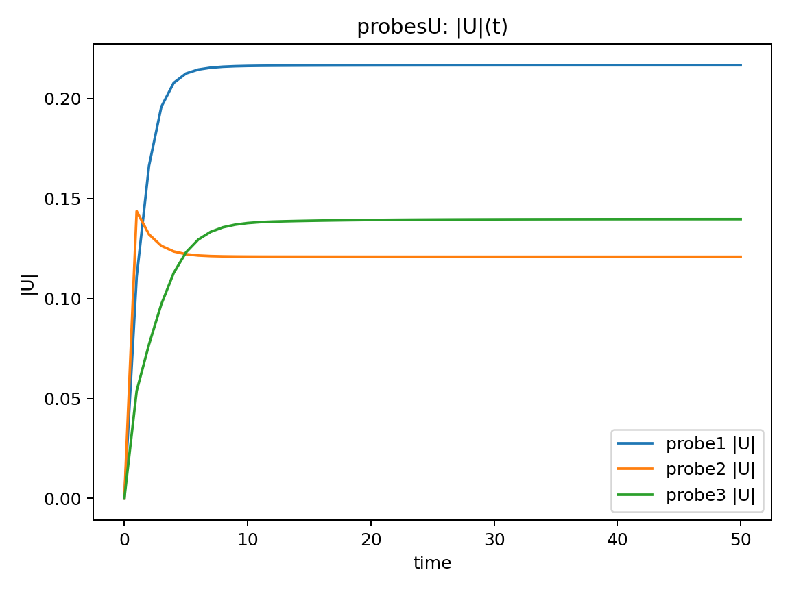
- 各 probe の $|U|(t)$ ($|U| = \sqrt{u^2 + v^2}$)
- 出力間隔ごとの max|ΔU|
を可視化する。
👇定常判定スクリプト
#!/usr/bin/env python3
# plot_steadiness_probesU.py
from pathlib import Path
import re
import numpy as np
import matplotlib.pyplot as plt

def read_probes_U(p):
    lines = [l for l in p.read_text().splitlines()
             if l.strip() and not l.lstrip().startswith("#")]
    ts, Us = [], []
    for l in lines:
        nums = [float(x) for x in re.findall(r"[-+]?\d*\.?\d+(?:[eE][-+]?\d+)?", l)]
        t = nums[0]
        vals = np.array(nums[1:])
        U = vals.reshape(-1, 3)
        ts.append(t)
        Us.append(U)
    return np.array(ts), np.stack(Us)

p = Path("postProcessing/probesU/0/U")
t, U = read_probes_U(p)
Umag = np.linalg.norm(U, axis=2)

# |U|(t)
plt.figure()
for i in range(Umag.shape[1]):
    plt.plot(t, Umag[:, i], label=f"probe{i+1}")
plt.xlabel("time")
plt.ylabel("|U|")
plt.legend()
plt.title("Velocity magnitude at probes")
plt.savefig("steady_probesU_timeseries.png", dpi=150)
plt.close()

# max |ΔU|
d = np.abs(np.diff(Umag, axis=0))
plt.figure()
plt.plot(t[1:], d.max(axis=1))
plt.yscale("log")
plt.xlabel("time")
plt.ylabel("max |ΔU|")
plt.title("Max velocity change between outputs")
plt.savefig("steady_probesU_delta.png", dpi=150)
plt.close()
13.2 定常到達の確認
|U|(t)について
初期は過渡的に変化ある時刻以降,3点すべてで $|U|$ がほぼ一定
→ 計算終了時は定常状態であると考えられます。
max|ΔU|について
出力間隔ごとの速度変化量を評価$max|ΔU|$ は時間とともに減少し,最終的に十分小さな値で頭打ちとなる以上より,計算終了時は定常解に収束したと考えられます。
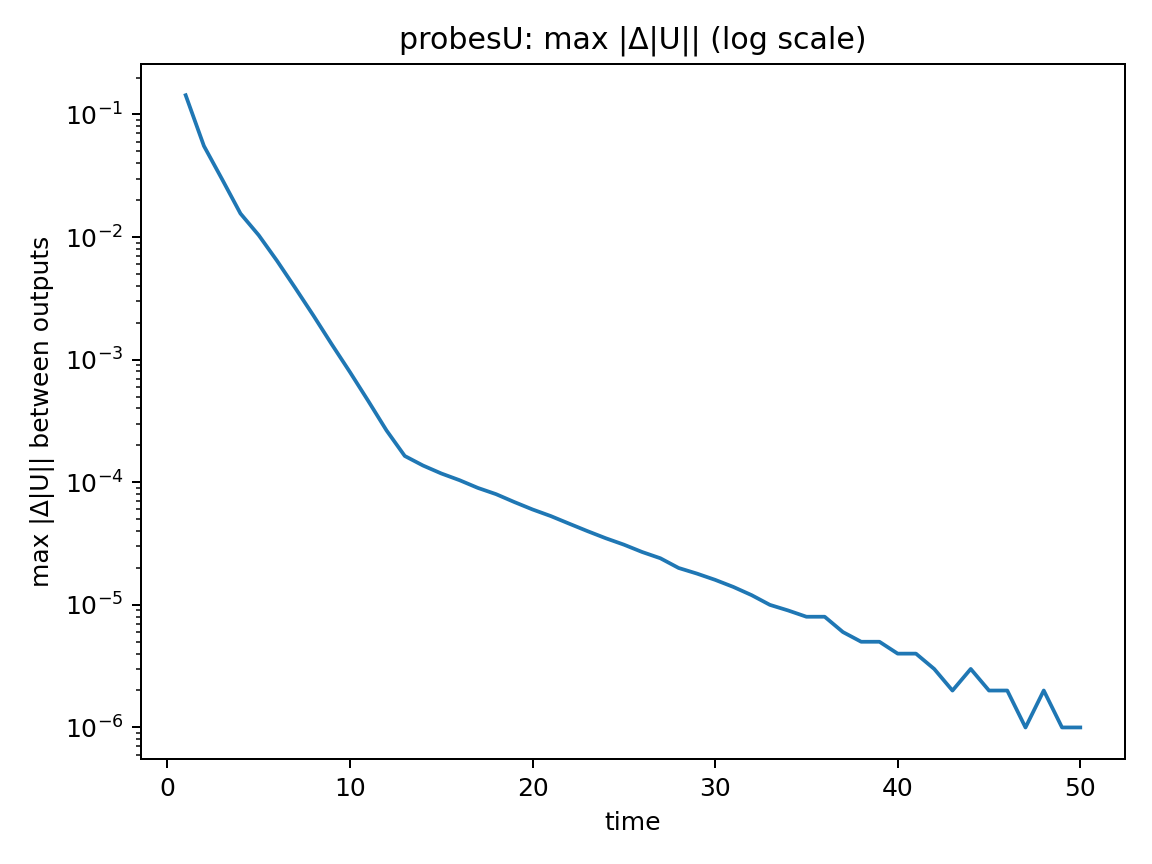
なお、ここでの time は非定常現象の再現が目的ではなく、定常解に収束させるための疑似時間として扱っています。
14. Ghia Table I/II と比較
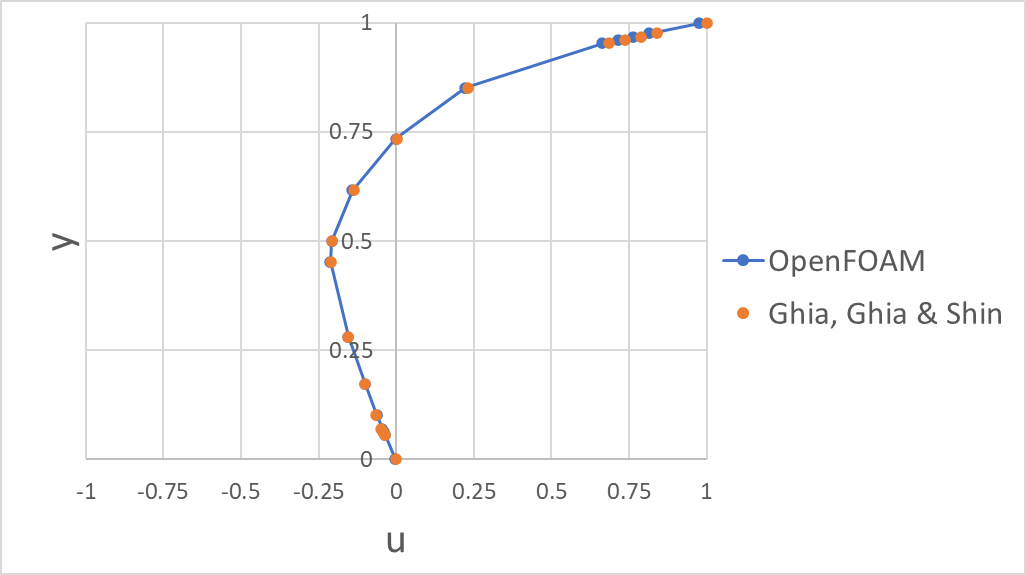
Ghia, Ghia & Shin[1]の Table I / II に記載の$u$, $v$の中心線流速分布との比較によるRMSEの結果は以下であり、良好な一致が見られました。なお、RMSEはGhia Table I/II に掲載された17点(境界点含む)で算出しました。また計算はExcelで RMSE = SQRT(AVERAGE((シミュレーション結果 - Ghia, Ghia & Shin[1]の結果)^2)) として算出しました。
- $u$のRMSE:$1.85495 \times 10^{-4}$
- $v$のRMSE: $4.26789 \times 10^{-5}$
ただし、$u$のところについて、y=1の壁が駆動しているところの値が$u=1$とならなかったり、y=0でno slipのところの値が$u=0$にならないということが見られました($v$についても同様)。これは境界(patch face)上の値そのものではなく、probesが返す補間値(内部寄りの評価値)を比較している可能性があると考えています。 この点については次回以降の記事で改善に取り組もうと思います。
またそれぞれの結果をプロットした結果が以下です。
👇:Table I に記載の$u$の中心線速度分布との比較プロット(凡例のOpenFOAMは本記事での結果、Ghia, Ghia & Shinは参考文献[1]の結果)
👇:Table II に記載の$v$の中心線速度分布(凡例のOpenFOAMは本記事での結果、Ghia, Ghia & Shinは参考文献[1]の結果)

15. ParaViewでStreamlineを表示する(背景コンター無し+外形あり)
15.1 起動
paraFoam
15.2 2D表示用にSliceを作る
Pipeline Browser で ...OpenFOAM を選択した後にあとで以下の項目を順番に選択していきます。
- Filters → Slice
👇 - Normal: (0,0,1)
👇 - Origin: (0,0,0.05)(厚み0〜0.1想定の中央)
👇 - Apply
15.3 外形(枠線)だけ出す(Outline)
- Slice1 を選択
👇 - Filters → Outline
👇 - Apply
表示(👁)は Outline1をON、Slice1はOFF(塗りつぶしを消す)
15.4 Stream Tracer(流線の表示方法)
以下の項目を順番に選択していきます。
- Slice1 を選択
👇 - Filters → Stream Tracer
👇 - Vectors: U
👇 - Seed Type: Line
👇 - Point1: (0, 0, 0.05)
- Point2: (1, 1, 0.05)
- Resolution: 50(本数)
- Integration Direction: BOTH(あれば選択)
👇 - Apply
またその他以下の設定とする。
- Outline1:ON(外形)
- StreamTracer1:ON(流線)
- Slice1:OFF(塗りつぶし不要)
- (Glyphは必要ならON)
16. Streamlineを動画化(PNG連番 → mp4)
16.1 framesフォルダ作成
mkdir -p frames
16.2 ParaViewでPNG連番を書き出す
以下の項目を順番に選択していきます。
- File → Save Animation…
👇 - File name:frames/streamline.png
👇 - Resolution:1920 × 1080(※H.264の都合で偶数推奨)
frames/streamline.0036.png のような連番のpngが保存される
16.3 ffmpegをインストール(無ければ)
sudo apt-get update
sudo apt-get install -y ffmpeg
16.4 連番の開始番号を確認
ls -1 frames | head -n 5
例:streamline.0036.png が最初なら start_number=36。
16.5 mp4化
以下のコマンドで出力されたpngファイルを動画化しました。
ffmpeg -framerate 1 -start_number 36 -i frames/streamline.%04d.png -c:v libx264 -pix_fmt yuv420p cavity_streamline.mp4
このようにして作成した動画が以下になります
17. まとめ
OpenFOAM-11 の2D lid-driven cavity flowケースを Re = 100 の層流条件で計算し,Ghia, Ghia & Shin[1] によって示されている中心線速度分布(Table I / II)との比較を行いました。本環境では sample/sets が使用できないケースがあったため,確実に動作する probes を用いて,中心線上の 129 点 × 2 本の速度データを取得しました。得られた結果は ParaView で Streamline を可視化し,PNG の連番画像から ffmpeg を用いて mp4 動画を生成しました。なお,解像度は 1920×1080 とすることで,エンコード時の問題を回避しています。
Ghia, Ghia & Shin[1] の Table I / II に記載されている中心線速度分布($u$, $v$)との比較から算出した RMSE は,全体として良好な一致を示しました。一方で,$u$ 成分については,駆動壁に対応する $y=1$ で $u=1$ とならない点や,no-slip 条件を課している $y=0$ で $u=0$ とならない点が確認されました($v$ 成分についても同様の傾向が見られます)。これらの差異は,速度の定義位置(計算点)の違いに起因するものと考えられます。この点については,今後の記事で改善を検討していく予定です。
参考文献
[1] Ghia, U., K. N. Ghia, and C. T. Shin. 1982. “High-Re Solutions for Incompressible Flow Using the Navier–Stokes Equations and a Multigrid Method.” Journal of Computational Physics 48 (3): 387–411. https://doi.org/10.1016/0021-9991(82)90058-4.