1. はじめに
前回の記事ではRe=100で2D lid-driven cavity flow(浮力なし) を対象としてシミュレーションをしましたが、本記事ではRe = 400 の流れを OpenFOAM-11 を用いて数値シミュレーションしてみました。
実施した内容は前回の記事とは変わりませんので、前回との違いと前回の記事で構築した環境のどこを変えればよいかにスポットを当てて記事を書いていきます。(ほとんどの手順は前回と一緒ですが、手順を書き残すという意味でもこの記事でも書きます)
2. 実行環境
- CPU: CORE i7 7th Gen
- メモリ: 32GB
- GPU: GeForce RTX 2070
- OS: Ubuntu22.04(WSL2ではなくPCに直接インストール)
3. OpenFOAM環境の読み込み
OpenFOAMの環境変数を有効化:
source ~/OpenFOAM/OpenFOAM-11/etc/bashrc
$FOAM_RUNが使えることを確認:
echo $FOAM_RUN
4. チュートリアルケースを複製(Re=400用)
元ケースを壊さないように 前回作成したRe=100のケースを複製して作業していきます。
cd $FOAM_RUN
cp -r cavity_Ghia_Re100 cavity_Ghia_Re400
cd cavity_Ghia_Re400
5. 2D lid-driven cavity の前提確認(境界条件)
OpenFOAMでは、front/back 面を empty に設定し、厚み方向セル数を 1 にすることで「2次元問題」として解いていきます。前回の記事で既に設定はしていますが、ここでは 0/U の上壁が (1 0 0)、側壁・底が noSlip、front/back が empty になっていることを確認していきます。
cat 0/U
cat 0/p
*結果は以下と同じであることを確認します👇
6. 層流化(laminar)
Ghia(1982)は2次元層流条件の基準データなので、乱流モデルをOFFにします。
constant/momentumTransport を laminar のみにします:
cat > constant/momentumTransport << 'EOF'
FoamFile
{
    format      ascii;
    class       dictionary;
    location    "constant";
    object      momentumTransport;
}
simulationType  laminar;
EOF
7. Re=400 に合わせる(U=1, L=1)
7.1 convertToMeters を 1 にして L=1 にする
system/blockMeshDict の convertToMeters を確認:
grep -n "convertToMeters" -n system/blockMeshDict
必要なら置換します:
sed -i 's/convertToMeters.*/convertToMeters 1;/' system/blockMeshDict
7.2 nu を Re=400 に(nu = 1/400 = 0.0025)
constant/physicalProperties を編集:
cat > constant/physicalProperties << 'EOF'
FoamFile
{
    format      ascii;
    class       dictionary;
    location    "constant";
    object      physicalProperties;
}

viscosityModel  constant;

nu              [0 2 -1 0 0 0 0] 0.0025;
EOF
以下のコマンドで確認します:
grep -n "nu" constant/physicalProperties
8. メッシュを 128×128×1 にする
Ghia(1982)の Table I/II に列挙されている座標は 1/128 系の点が多いため、ここでは 128×128×1 を採用する。
system/blockMeshDict の該当行を確認:
grep -n "hex" -n system/blockMeshDict
blocks を次のようにします。(手作業で編集しました):
hex (0 1 2 3 4 5 6 7) (128 128 1) simpleGrading (1 1 1)
9. fvSchemes(今回使用したもの)
今回使用した system/fvSchemes は以下です(Re=400でもまず安定寄りで回す)。
※div(phi,k) 等の乱流用スキームが残っているが、laminarでは k/epsilon 等の方程式を解かないため参照されません。
ddtSchemes
{
    default         Euler;
}

gradSchemes
{
    default         Gauss linear;
}

divSchemes
{
    default         none;
    div(phi,U)      Gauss limitedLinearV 1;
    div(phi,k)      Gauss limitedLinear 1;
    div(phi,epsilon) Gauss limitedLinear 1;
    div(phi,omega)  Gauss limitedLinear 1;
    div(phi,R)      Gauss limitedLinear 1;
    div(R)          Gauss linear;
    div(phi,nuTilda) Gauss limitedLinear 1;
    div((nuEff*dev2(T(grad(U))))) Gauss linear;
}

laplacianSchemes
{
    default         Gauss linear corrected;
}

interpolationSchemes
{
    default         linear;
}

snGradSchemes
{
    default         corrected;
}
10. controlDict(タイムステップと出力間隔)
今回もdeltaT=0.01、writeInterval=100 とし、1秒ごとに結果を出力しました。
cat > system/controlDict << 'EOF'
FoamFile
{
    format      ascii;
    class       dictionary;
    location    "system";
    object      controlDict;
}

application     foamRun;
solver          incompressibleFluid;

startFrom       startTime;
startTime       0;

stopAt          endTime;
endTime         50;

deltaT          0.01;

writeControl    timeStep;
writeInterval   100;

purgeWrite      0;

writeFormat     ascii;
writePrecision  6;
writeCompression off;

timeFormat      general;
timePrecision   6;

runTimeModifiable true;
EOF
11. 定常判定&中心線取得のための probes
本環境では foamPostProcess -func sample を実行すると "Cannot find configuration file sample" が出たため、本記事では functionObject probes を用いて、中心線 129点×2本(計258点 x方向とy方向に1本ずつ)を時系列として出力しました。
11.1 重要:probesが返す値について(本記事の前提)
OpenFOAMでは U はセル中心(volVectorField)に定義され、probes は指定座標での値を返す際に セル中心場から補間して点値を出力します。そのため、特に境界上(y=0,1 など)の点では、境界面の固定値そのものではなく「内部寄りの補間値」が出力されます。本記事では、この性質を前提に 中心線分布の再現性(主に内部点) を確認します。
11.2 中心線プローブ点(258点)をPythonで自動生成
以下を実行して出力をコピーします(z=0.05は厚み0〜0.1の中央):
python3 - << 'PY'
import numpy as np

z = 0.05
n = 129

ys = np.linspace(0, 1, n)
xs = np.linspace(0, 1, n)

print("        probeLocations")
print("        (")
# u(x=0.5,y)
for y in ys:
    print(f"            (0.5 {y:.8f} {z})")
# v(x,y=0.5)
for x in xs:
    print(f"            ({x:.8f} 0.5 {z})")
print("        );")
PY
11.3 system/controlDict に functions を追記(probesU + centerLineProbes)
※functions { ... } が既にある場合は、追記ではなく編集して1つにまとめます。
cat >> system/controlDict << 'EOF'

functions
{
    // --- (A) 定常判定用:3点 ---
    probesU
    {
        type            probes;
        libs            ("libsampling.so");

        writeControl    timeStep;
        writeInterval   100;

        fields          (U);

        probeLocations
        (
            (0.5 0.5 0.05)
            (0.5 0.75 0.05)
            (0.5 0.25 0.05)
        );
    }

    // --- (B) Ghia比較用:中心線 129点×2本 ---
    centerLineProbes
    {
        type            probes;
        libs            ("libsampling.so");

        writeControl    timeStep;
        writeInterval   100;

        fields          (U);

        // ★ここに「11.2で生成した probeLocations ブロック」を貼り付けます★
    }
}
EOF
反映確認:
foamDictionary system/controlDict -entry functions -value
12. メッシュ生成→計算実行
foamCleanCase
rm -rf constant/polyMesh
blockMesh
checkMesh
foamRun
13. 定常になったかの確認(probes)
13.1 定常判定の可視化(Python)
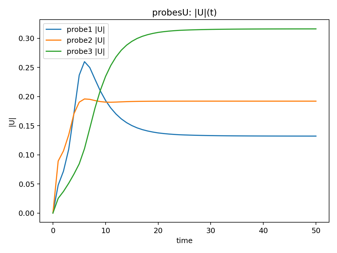
各probe点の $|U|(t)$ と、出力間隔ごとの max|ΔU| を確認する。
なお、$|U|$は$|U| = \sqrt{u^2 + v^2}$(合成流速)
#!/usr/bin/env python3
# plot_steadiness_probesU.py
from pathlib import Path
import re
import numpy as np
import matplotlib.pyplot as plt

def read_probes_U(p):
    lines = [l for l in p.read_text().splitlines()
             if l.strip() and not l.lstrip().startswith("#")]
    ts, Us = [], []
    for l in lines:
        nums = [float(x) for x in re.findall(r"[-+]?\d*\.?\d+(?:[eE][-+]?\d+)?", l)]
        t = nums[0]
        vals = np.array(nums[1:])
        U = vals.reshape(-1, 3)
        ts.append(t)
        Us.append(U)
    return np.array(ts), np.stack(Us)

p = Path("postProcessing/probesU/0/U")
t, U = read_probes_U(p)
Umag = np.linalg.norm(U, axis=2)

plt.figure()
for i in range(Umag.shape[1]):
    plt.plot(t, Umag[:, i], label=f"probe{i+1}")
plt.xlabel("time")
plt.ylabel("|U|")
plt.legend()
plt.title("Velocity magnitude at probes")
plt.savefig("steady_probesU_timeseries.png", dpi=150)
plt.close()

d = np.abs(np.diff(Umag, axis=0))
plt.figure()
plt.plot(t[1:], d.max(axis=1))
plt.yscale("log")
plt.xlabel("time")
plt.ylabel("max |ΔU|")
plt.title("Max velocity change between outputs")
plt.savefig("steady_probesU_delta.png", dpi=150)
plt.close()
実行:
python3 plot_steadiness_probesU.py
13.2 定常到達の確認
|U|(t)について
初期は過渡的に変化ある時刻以降,3点すべてで $|U|$ がほぼ一定
→ 計算終了時は定常状態であると考えられます。
max|ΔU|について
出力間隔ごとの速度変化量を評価$max|ΔU|$ は時間とともに減少し,最終的に十分小さな値で頭打ちとなっています。以上のことより,計算終了時は定常解に収束したと考えられます。
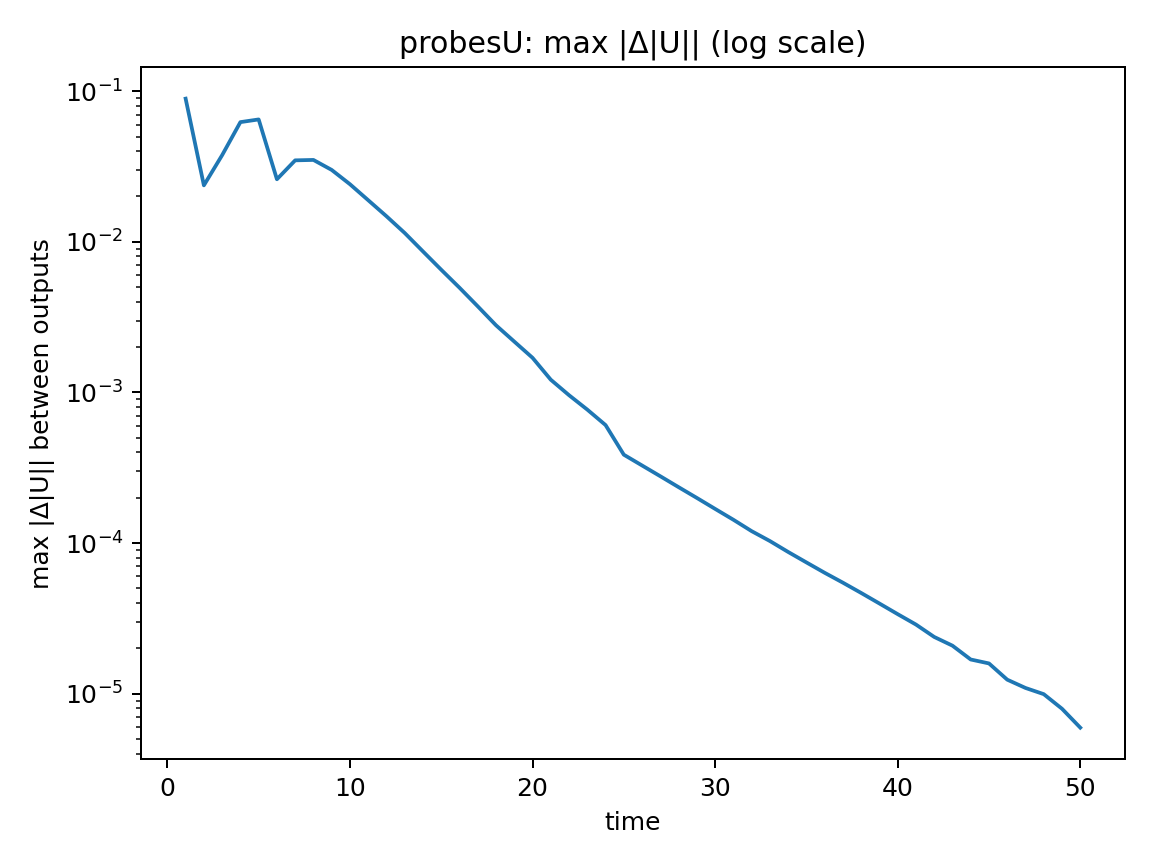
なお、ここでの time は非定常現象の再現が目的ではなく、定常解に収束させるための疑似時間として扱っています。
14. Ghia Table I/II と比較
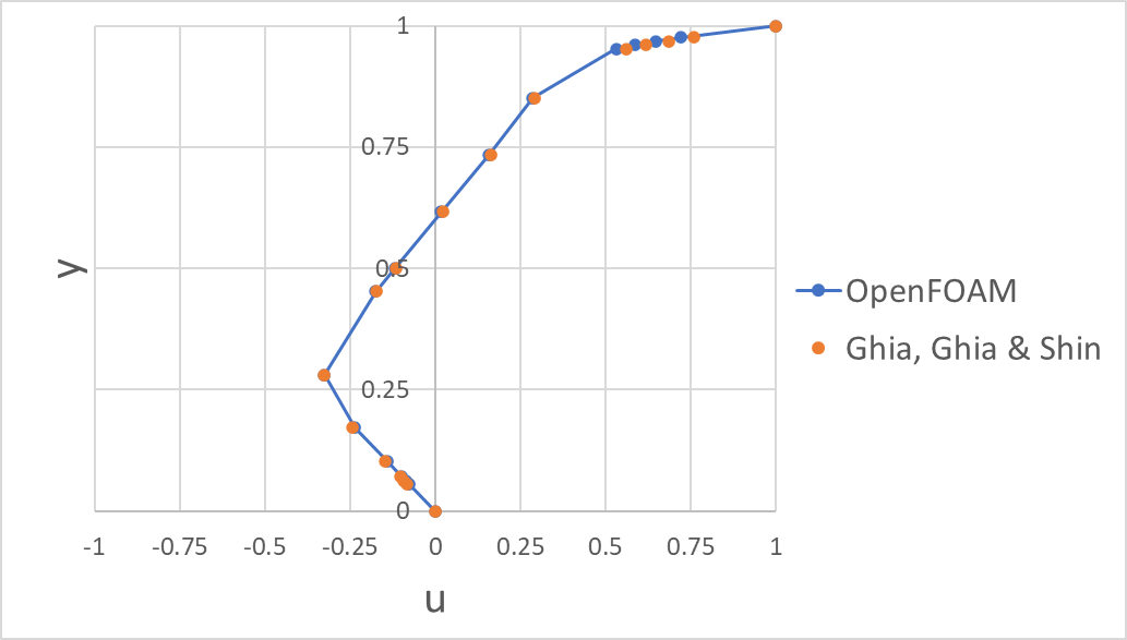
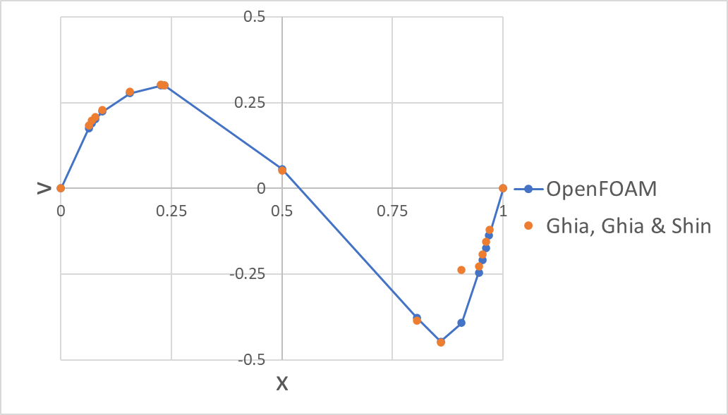
Ghia, Ghia & Shin[1]の Table I / II に記載の$u$, $v$の中心線流速分布との比較によるRMSEの結果は以下であり、良好な一致が見られました。なお、RMSEはGhia Table I/II に掲載された17点(境界点含む)で算出しました。また計算はExcelで RMSE = SQRT(AVERAGE((シミュレーション結果 - Ghia, Ghia & Shin[1]の結果)^2)) として算出しました。
- $u$のRMSE:$3.35505\times 10^{-4}$
- $v$のRMSE: $1.582108\times 10^{-3}$
※境界点(y=0,1 / x=0,1)はprobesが返す補間値でしたため、計算からは除外しています。
👇:Table I に記載の$u$の中心線速度分布との比較プロット(凡例のOpenFOAMは本記事での結果、Ghia, Ghia & Shinは参考文献[1]の結果)
👇:Table II に記載の$v$の中心線速度分布(凡例のOpenFOAMは本記事での結果、Ghia, Ghia & Shinは参考文献[1]の結果)
15. 流線(streamline)の可視化
以下の記事で示した手順で作成した動画が以下になります
右下領域の流線(streamline)が十分に描画されておらず、可視化手法の修正が必要と思われます。
16. まとめ
OpenFOAM-11 を用いて,2 次元 lid-driven cavity 流れ(Re=400,層流)の数値計算を行いました。計算結果から probes を用いて中心線上の速度成分を取得し,129 点 × 2 本のデータとして,Ghia, Ghia & Shin (1982)[1] に示されている Table I / II(Re=400)と比較しました。なお,probes はセル中心値から補間した点値を出力する仕様であるため,$y=0,1$ などの境界点では,境界条件として与えた固定値そのものは取得できません。このため,これらの境界点は比較対象から除外しています。
以上の条件のもとで,Ghia, Ghia & Shin[1] の Table I / II に示されている中心線速度分布($u$, $v$)との比較を行い,その結果から算出した RMSE は,全体として良好な一致を示しました。
一方で,流線(streamline)の可視化において,右下領域の流線が十分に描画されていない箇所が確認されました。これは可視化条件や描画手法に起因する可能性があるため,今後は OpenFOAM における描画設定の変更などの可視化手法を検討し,流れ場全体をより適切に表現できる方法を模索していきたいと考えています。
参考文献
[1] Ghia, U., K. N. Ghia, and C. T. Shin. 1982. “High-Re Solutions for Incompressible Flow Using the Navier–Stokes Equations and a Multigrid Method.” Journal of Computational Physics 48 (3): 387–411. https://doi.org/10.1016/0021-9991(82)90058-4.
.