
はじめに
生成AIによって、人類の知は向上するのだろうか?
生成AIは人類の敵なのか。それとも、救世主となり得るのだろうか。
生成AIは、人類が生み出した膨大なデータの平均値付近の値を出力するというアルゴリズムで動いている。
したがって、人類が自分の頭でデータを生み出さず、生成AIで新しいデータを作ってばかりいたら将来的に、
人類の知であるデータの質はどのようになるのだろうか。
今回は、そのようなモデルをPython,Claudeで作成し、シミュレーションを行った。
そして、単一社会になりつつある現代を生きる上で、人類ができることについて、多様性という観点から考察した。
ただし、Claudeで生成したプログラムは巻末に全文を示した。

シミュレーションモデル
生成AIによって新しいデータが次々に生成されていく場合、データの質は量が増加するにつれてどのように変化するか、モデルを作成してシミュレーションをした。
・初期条件は$n$個の正規分布に従うデータセットがあるとする。
(ただし、標準偏差はシグマで平均は0とし、$n=100$程度と考えた。)
・1回の試行で、データセットの平均付近で標準偏差が$\frac{\sigma}{a}$ を満たすデータを1つ生成し、データセットに追加する。
・$a=3$程度の定数とみなした場合と$a=kn$($n$は現時点のデータセットのデータ数)とする場合で結果がどのように変化するのか調査した。
この操作を$mn$(mは10程度の大きな整数)まで実施した場合のデータセットの分布の変化を観測した。
具体的には、以下のアウトプットを出力できるプログラムを作成した。
・分布の推移について代表的な動きがわかる程度でgif動画化する
・平均と標準偏差の推移も観測したい。(おそらくデータセットのデータ数が増えるほど平均が0に漸近し、標準偏差も0付近になるか?)
計算条件
初期のデータセットのデータ数を$n=100$とし、以下の場合シミュレーションを実施した。
a=3(定数)のとき
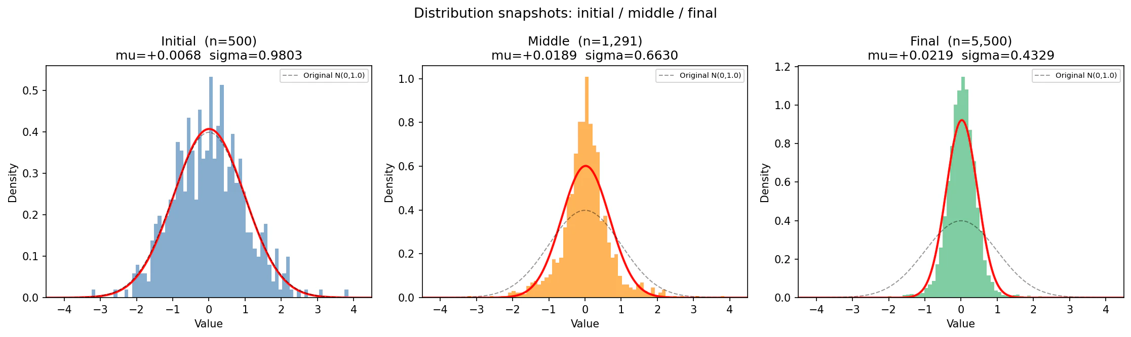
この場合は、標準偏差が1から$0.33$に向かってゆるやかに小さくなるような推移を示した。
このことから、多様性が世代を追うごとに失われていく。ただし、標準偏差は0とならないところが、興味深いところである。
動画

推移

参考に、$a=10$の場合の結果を以下に示す。$a=3$の場合と比較して急激に標準偏差が低下している。
動画
推移

a=knのとき
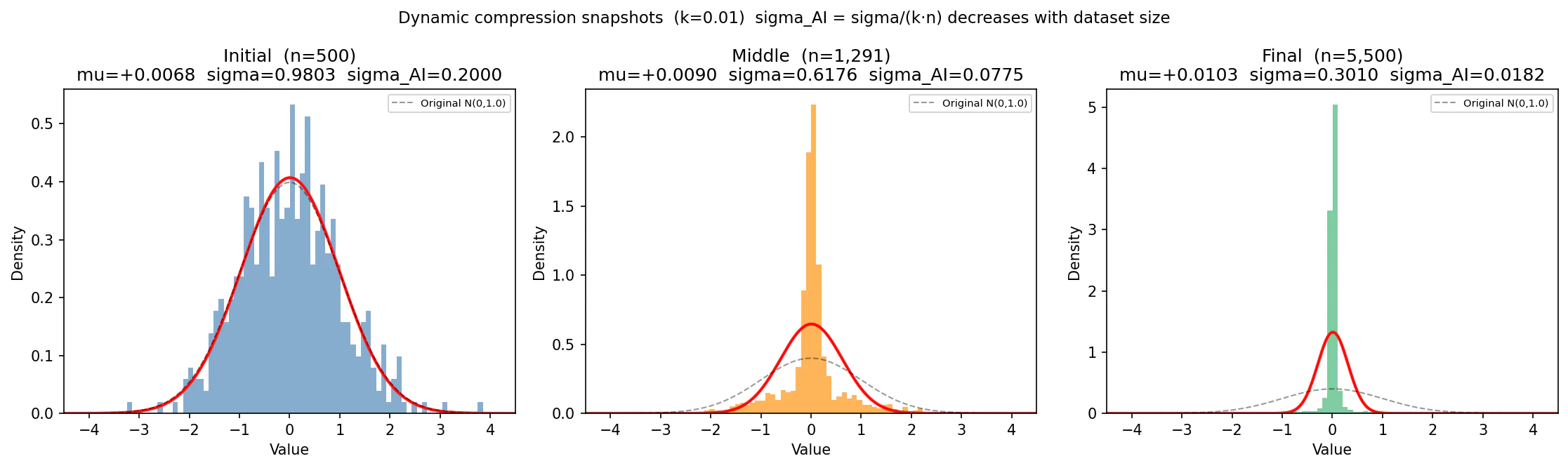
$k=0.01$での結果を以下に示す。急激に標準偏差が0に漸近するような極端な結果となった。
今回怖いのが、$a$に値の制限を付けなかったため、標準偏差がいくらでも0に近づけられるという点である。
動画
推移
考察
以上の結果より、ランダムさ(多様性)が失われることが、AI社会にとって深刻な問題となる可能性があることが分かった。人類が生成$AI$よりも優れている点は、
・リアルかつ最先端の情報を生み出せる。
・個人の体験やノウハウなど曖昧なものを表現できる。
・データが少ない専門の知識を扱える
といった点が挙げられる。また、人間の特徴として、
・多様性がある。
・間違いが多い
といったことが挙げられる。
多様性があり、間違いが多いというのは、現代社会(モノカルチャー的な社会)ではマイナスなことに一見思えるが、将来のことを考えると、データのばらつきを増やすという貴重な価値を提供する原動力となる。
もちろん、多様性を求めすぎても社会の秩序は崩壊してしまう。だが、生成AIを上手に人間が活用し、制御することで、多様性のある面白い社会を作り出すことは可能であると信じたい。
まとめ
今回は、生成AIが社会に与える、データの平均化について考察した。
その影響は、下手をすると数年後に単一化社会として顕在化するかもしれない。
それまでに我々、人類ができることは、単調な作業は、生成AIに任せて創造的な活動をすることだと考えられる。
そのためには、多様な書籍や質の良い情報に触れ、適宜にアウトプットし、生成AIをあくまで成長の道具として活用することが重要となる。
プログラム
a=3(定数)のとき
#!/usr/bin/env python3
"""
Simulation: How distribution changes as AI-generated data accumulates

Initial dataset : n samples from N(0, sigma)
Each step       : generate 1 point from N(current_mean, sigma/a), add to dataset
Repeat          : m*n times total
Output          : GIF animation + snapshot PNG
"""

import numpy as np
import matplotlib.pyplot as plt
import matplotlib.animation as animation
from scipy.stats import norm

# ============================================================
# Parameters
# ============================================================
n = 500        # initial dataset size
sigma = 1.0    # initial standard deviation
a = 3.0        # compression factor (a > 1); AI-generated data has std = sigma/a
m = 10         # step multiplier (total additions = m*n)

RANDOM_SEED = 42
OUTPUT_GIF = "distribution_evolution.gif"
OUTPUT_PNG = "distribution_snapshots.png"

# ============================================================
# Simulation
# ============================================================
np.random.seed(RANDOM_SEED)
total_additions = m * n

# Initial dataset from N(0, sigma)
data = list(np.random.normal(0, sigma, n))
running_sum = float(sum(data))

# Frame selection: dense at start (visible early changes), sparse later
early = list(range(0, min(300, total_additions + 1), 30))
late  = list(np.logspace(np.log10(max(300, 1)), np.log10(total_additions), 30).astype(int))
frame_set = set([0] + early + late + [total_additions])

history = []

def record(step, data_list, rsum):
    arr = np.array(data_list)
    history.append({
        'step': step,
        'total_n': len(arr),
        'mean': rsum / len(arr),
        'std': float(arr.std()),
        'data': arr.copy(),
    })

record(0, data, running_sum)

print("Running simulation...")
for step in range(1, total_additions + 1):
    current_mean = running_sum / len(data)
    new_pt = float(np.random.normal(current_mean, sigma / a))
    data.append(new_pt)
    running_sum += new_pt

    if step in frame_set:
        record(step, data, running_sum)

    if step % (total_additions // 5) == 0:
        m_val = running_sum / len(data)
        s_val = np.std(data)
        print(f"  step {step:>6}/{total_additions}  n={len(data):>5}  "
              f"mean={m_val:+.4f}  std={s_val:.4f}")

print(f"Done. Frames recorded: {len(history)}")

# ============================================================
# Animation
# ============================================================
fig = plt.figure(figsize=(13, 8))
fig.suptitle(
    f"Effect of accumulating AI-generated data  "
    f"(initial n={n}, sigma={sigma}, a={a}, m={m})",
    fontsize=11
)
gs = fig.add_gridspec(2, 2, hspace=0.48, wspace=0.35)
ax_hist = fig.add_subplot(gs[0, :])
ax_mean = fig.add_subplot(gs[1, 0])
ax_std  = fig.add_subplot(gs[1, 1])

x_range = np.linspace(-4.5 * sigma, 4.5 * sigma, 500)
all_ns   = [h['total_n'] for h in history]
all_mean = [h['mean']    for h in history]
all_std  = [h['std']     for h in history]

mean_pad = sigma * 0.35
mean_ylim = (min(-mean_pad, min(all_mean) * 1.3), max(mean_pad, max(all_mean) * 1.3))
std_ylim  = (0.0, sigma * 1.25)

def update(i):
    h = history[i]
    xs = [h2['total_n'] for h2 in history[:i+1]]

    # ---- Distribution histogram ----
    ax_hist.clear()
    ax_hist.hist(h['data'], bins=70, density=True,
                 alpha=0.6, color='steelblue', edgecolor='none', label='Data')
    ax_hist.plot(x_range, norm.pdf(x_range, h['mean'], h['std']),
                 'r-', lw=2,
                 label=f"Fit  mu={h['mean']:+.4f}  sigma={h['std']:.4f}")
    # Reference: original N(0, sigma)
    ax_hist.plot(x_range, norm.pdf(x_range, 0, sigma),
                 'k--', lw=1, alpha=0.4, label=f"Original N(0,{sigma})")
    ax_hist.set_xlim(-4.5*sigma, 4.5*sigma)
    ax_hist.set_ylim(bottom=0)
    ax_hist.set_title(
        f"Distribution  |  total data points: {h['total_n']:,}  "
        f"(+{h['step']:,} AI-generated)"
    )
    ax_hist.set_xlabel("Value")
    ax_hist.set_ylabel("Density")
    ax_hist.legend(loc='upper right', fontsize=8)

    # ---- Mean evolution ----
    ax_mean.clear()
    ax_mean.plot(xs, [h2['mean'] for h2 in history[:i+1]],
                 'b-', lw=1.8, zorder=3)
    ax_mean.axhline(0, color='red', ls='--', lw=1, alpha=0.7, label='True mean = 0')
    ax_mean.scatter([xs[-1]], [h['mean']], s=40, color='blue', zorder=5)
    ax_mean.set_xlim(n, n + total_additions)
    ax_mean.set_ylim(*mean_ylim)
    ax_mean.set_title("Mean over time")
    ax_mean.set_xlabel("Total data points")
    ax_mean.set_ylabel("Mean")
    ax_mean.legend(fontsize=8)

    # ---- Std evolution ----
    ax_std.clear()
    ax_std.plot(xs, [h2['std'] for h2 in history[:i+1]],
                'g-', lw=1.8, zorder=3)
    ax_std.axhline(sigma,   color='red',    ls='--', lw=1, alpha=0.7,
                   label=f'Initial sigma = {sigma}')
    ax_std.axhline(sigma/a, color='orange', ls='--', lw=1, alpha=0.8,
                   label=f'AI sigma = {sigma/a:.3f}')
    ax_std.scatter([xs[-1]], [h['std']], s=40, color='green', zorder=5)
    ax_std.set_xlim(n, n + total_additions)
    ax_std.set_ylim(*std_ylim)
    ax_std.set_title("Std deviation over time")
    ax_std.set_xlabel("Total data points")
    ax_std.set_ylabel("Std deviation")
    ax_std.legend(fontsize=8)

print("Generating GIF animation...")
ani = animation.FuncAnimation(fig, update, frames=len(history),
                              interval=300, repeat=True)
ani.save(OUTPUT_GIF, writer='pillow', fps=4)
print(f"Saved: {OUTPUT_GIF}")
plt.close(fig)

# ============================================================
# Snapshot comparison (initial / middle / final)
# ============================================================
fig2, axes = plt.subplots(1, 3, figsize=(15, 4.5))
fig2.suptitle("Distribution snapshots: initial / middle / final", fontsize=13)

idx_mid = len(history) // 2
snaps   = [history[0], history[idx_mid], history[-1]]
colors  = ['steelblue', 'darkorange', 'mediumseagreen']
labels  = ['Initial', 'Middle', 'Final']

for ax, h, color, label in zip(axes, snaps, colors, labels):
    ax.hist(h['data'], bins=70, density=True,
            alpha=0.65, color=color, edgecolor='none')
    ax.plot(x_range, norm.pdf(x_range, h['mean'], h['std']), 'r-', lw=2)
    ax.plot(x_range, norm.pdf(x_range, 0, sigma), 'k--', lw=1,
            alpha=0.4, label=f'Original N(0,{sigma})')
    ax.set_xlim(-4.5*sigma, 4.5*sigma)
    ax.set_ylim(bottom=0)
    ax.set_title(
        f"{label}  (n={h['total_n']:,})\n"
        f"mu={h['mean']:+.4f}  sigma={h['std']:.4f}"
    )
    ax.set_xlabel("Value")
    ax.set_ylabel("Density")
    ax.legend(fontsize=7)

plt.tight_layout()
plt.savefig(OUTPUT_PNG, dpi=150, bbox_inches='tight')
print(f"Saved: {OUTPUT_PNG}")
plt.close(fig2)

# ============================================================
# Summary
# ============================================================
final = history[-1]
print("\n=== Final state summary ===")
print(f"  Total data points : {final['total_n']:,}")
print(f"  Mean              : {final['mean']:+.6f}  (target: 0)")
print(f"  Std deviation     : {final['std']:.6f}  "
      f"(initial: {sigma}, AI: {sigma/a:.4f})")
print(f"\nFiles: {OUTPUT_GIF}, {OUTPUT_PNG}")
a=knのとき
$k=0.01$程度とした。
#!/usr/bin/env python3
"""
Simulation with DYNAMIC compression factor:
  a(t) = k * current_n   (current_n = dataset size at step t)
  AI-generated data: N(current_mean, sigma / a(t))

As the dataset grows, a grows proportionally, making AI-generated data
increasingly tight around the current mean.
"""

import numpy as np
import matplotlib.pyplot as plt
import matplotlib.animation as animation
from scipy.stats import norm

# ============================================================
# Parameters
# ============================================================
n = 500        # initial dataset size
sigma = 1.0    # initial standard deviation
k = 0.01       # dynamic constant; a = k * current_n  (so initial a = k*n = 5)
m = 10         # step multiplier (total additions = m*n)

RANDOM_SEED = 42
OUTPUT_GIF = "distribution_evolution_dynamic.gif"
OUTPUT_PNG = "distribution_snapshots_dynamic.png"

# ============================================================
# Simulation
# ============================================================
np.random.seed(RANDOM_SEED)
total_additions = m * n

data = list(np.random.normal(0, sigma, n))
running_sum = float(sum(data))

# Frame selection: dense at start, sparse later
early = list(range(0, min(300, total_additions + 1), 30))
late  = list(np.logspace(np.log10(max(300, 1)), np.log10(total_additions), 30).astype(int))
frame_set = set([0] + early + late + [total_additions])

history = []

def record(step, data_list, rsum, a_val):
    arr = np.array(data_list)
    history.append({
        'step':     step,
        'total_n':  len(arr),
        'mean':     rsum / len(arr),
        'std':      float(arr.std()),
        'a':        a_val,
        'sigma_ai': sigma / a_val,
        'data':     arr.copy(),
    })

# Step 0
a0 = k * len(data)
record(0, data, running_sum, a0)

print(f"Running simulation (dynamic a = k*n, k={k})...")
print(f"  Initial a = {a0:.2f}, initial sigma_ai = {sigma/a0:.4f}")
print(f"  Final   a = {k*(n+total_additions):.2f}, final sigma_ai = {sigma/(k*(n+total_additions)):.4f}")
print()

for step in range(1, total_additions + 1):
    current_n   = len(data)
    current_a   = k * current_n          # dynamic compression factor
    sigma_ai    = sigma / current_a
    current_mean = running_sum / current_n

    new_pt = float(np.random.normal(current_mean, sigma_ai))
    data.append(new_pt)
    running_sum += new_pt

    if step in frame_set:
        record(step, data, running_sum, current_a)

    if step % (total_additions // 5) == 0:
        mv = running_sum / len(data)
        sv = np.std(data)
        print(f"  step {step:>6}/{total_additions}  n={len(data):>5}  "
              f"mean={mv:+.4f}  std={sv:.4f}  "
              f"a={current_a:.2f}  sigma_ai={sigma_ai:.5f}")

print(f"\nDone. Frames recorded: {len(history)}")

# ============================================================
# Animation  (2 rows x 3 cols layout)
# ============================================================
fig = plt.figure(figsize=(15, 8))
fig.suptitle(
    f"Dynamic compression: a = k·n  (n=initial {n}, sigma={sigma}, k={k}, m={m})\n"
    f"sigma_AI = sigma / (k·n)  →  tightens automatically as dataset grows",
    fontsize=10
)
gs = fig.add_gridspec(2, 3, hspace=0.50, wspace=0.38)
ax_hist     = fig.add_subplot(gs[0, :])   # full-width top
ax_mean     = fig.add_subplot(gs[1, 0])
ax_std      = fig.add_subplot(gs[1, 1])
ax_sigma_ai = fig.add_subplot(gs[1, 2])

x_range = np.linspace(-4.5 * sigma, 4.5 * sigma, 500)

all_ns       = [h['total_n']  for h in history]
all_means    = [h['mean']     for h in history]
all_stds     = [h['std']      for h in history]
all_sigma_ai = [h['sigma_ai'] for h in history]

mean_pad  = sigma * 0.35
mean_ylim = (
    min(-mean_pad, min(all_means) * 1.3),
    max( mean_pad, max(all_means) * 1.3)
)
std_ylim  = (0.0, sigma * 1.25)
sai_ylim  = (0.0, max(all_sigma_ai) * 1.15)

def update(i):
    h  = history[i]
    xs = [h2['total_n'] for h2 in history[:i+1]]

    # ---- Distribution ----
    ax_hist.clear()
    ax_hist.hist(h['data'], bins=70, density=True,
                 alpha=0.6, color='steelblue', edgecolor='none', label='Data')
    ax_hist.plot(x_range, norm.pdf(x_range, h['mean'], h['std']),
                 'r-', lw=2,
                 label=f"Fit  mu={h['mean']:+.4f}  sigma={h['std']:.4f}")
    ax_hist.plot(x_range, norm.pdf(x_range, 0, sigma),
                 'k--', lw=1, alpha=0.35, label=f"Original N(0,{sigma})")
    ax_hist.set_xlim(-4.5*sigma, 4.5*sigma)
    ax_hist.set_ylim(bottom=0)
    ax_hist.set_title(
        f"Distribution  |  total points: {h['total_n']:,}  "
        f"(+{h['step']:,} AI-generated)  |  current a={h['a']:.2f}  sigma_AI={h['sigma_ai']:.4f}"
    )
    ax_hist.set_xlabel("Value")
    ax_hist.set_ylabel("Density")
    ax_hist.legend(loc='upper right', fontsize=8)

    # ---- Mean ----
    ax_mean.clear()
    ax_mean.plot(xs, [h2['mean'] for h2 in history[:i+1]], 'b-', lw=1.8, zorder=3)
    ax_mean.axhline(0, color='red', ls='--', lw=1, alpha=0.7, label='True mean = 0')
    ax_mean.scatter([xs[-1]], [h['mean']], s=40, color='blue', zorder=5)
    ax_mean.set_xlim(n, n + total_additions)
    ax_mean.set_ylim(*mean_ylim)
    ax_mean.set_title("Mean over time")
    ax_mean.set_xlabel("Total data points")
    ax_mean.set_ylabel("Mean")
    ax_mean.legend(fontsize=8)

    # ---- Std ----
    ax_std.clear()
    ax_std.plot(xs, [h2['std'] for h2 in history[:i+1]], 'g-', lw=1.8, zorder=3)
    ax_std.axhline(sigma, color='red', ls='--', lw=1, alpha=0.7,
                   label=f'Initial sigma = {sigma}')
    ax_std.scatter([xs[-1]], [h['std']], s=40, color='green', zorder=5)
    ax_std.set_xlim(n, n + total_additions)
    ax_std.set_ylim(*std_ylim)
    ax_std.set_title("Std deviation over time")
    ax_std.set_xlabel("Total data points")
    ax_std.set_ylabel("Std deviation")
    ax_std.legend(fontsize=8)

    # ---- sigma_AI (dynamic) ----
    ax_sigma_ai.clear()
    ax_sigma_ai.plot(xs, [h2['sigma_ai'] for h2 in history[:i+1]],
                     color='darkorange', lw=1.8, zorder=3)
    # Theoretical curve: sigma / (k * n)
    ns_theory = np.linspace(n, n + total_additions, 300)
    ax_sigma_ai.plot(ns_theory, sigma / (k * ns_theory),
                     'k--', lw=1, alpha=0.45, label=f'Theory: sigma/(k·n)')
    ax_sigma_ai.scatter([xs[-1]], [h['sigma_ai']], s=40, color='darkorange', zorder=5)
    ax_sigma_ai.set_xlim(n, n + total_additions)
    ax_sigma_ai.set_ylim(*sai_ylim)
    ax_sigma_ai.set_title("AI sigma (= sigma / a) over time")
    ax_sigma_ai.set_xlabel("Total data points")
    ax_sigma_ai.set_ylabel("sigma_AI")
    ax_sigma_ai.legend(fontsize=8)

print("Generating GIF animation...")
ani = animation.FuncAnimation(fig, update, frames=len(history),
                              interval=300, repeat=True)
ani.save(OUTPUT_GIF, writer='pillow', fps=4)
print(f"Saved: {OUTPUT_GIF}")
plt.close(fig)

# ============================================================
# Snapshot comparison (initial / middle / final)
# ============================================================
fig2, axes = plt.subplots(1, 3, figsize=(15, 4.5))
fig2.suptitle(
    f"Dynamic compression snapshots  (k={k})  "
    f"sigma_AI = sigma/(k·n) decreases with dataset size",
    fontsize=11
)

idx_mid = len(history) // 2
snaps  = [history[0], history[idx_mid], history[-1]]
colors = ['steelblue', 'darkorange', 'mediumseagreen']
labels = ['Initial', 'Middle', 'Final']

for ax, h, color, label in zip(axes, snaps, colors, labels):
    ax.hist(h['data'], bins=70, density=True,
            alpha=0.65, color=color, edgecolor='none')
    ax.plot(x_range, norm.pdf(x_range, h['mean'], h['std']), 'r-', lw=2)
    ax.plot(x_range, norm.pdf(x_range, 0, sigma), 'k--', lw=1,
            alpha=0.4, label=f'Original N(0,{sigma})')
    ax.set_xlim(-4.5*sigma, 4.5*sigma)
    ax.set_ylim(bottom=0)
    ax.set_title(
        f"{label}  (n={h['total_n']:,})\n"
        f"mu={h['mean']:+.4f}  sigma={h['std']:.4f}  sigma_AI={h['sigma_ai']:.4f}"
    )
    ax.set_xlabel("Value")
    ax.set_ylabel("Density")
    ax.legend(fontsize=7)

plt.tight_layout()
plt.savefig(OUTPUT_PNG, dpi=150, bbox_inches='tight')
print(f"Saved: {OUTPUT_PNG}")
plt.close(fig2)

# ============================================================
# Summary
# ============================================================
final = history[-1]
print("\n=== Final state summary ===")
print(f"  Total data points : {final['total_n']:,}")
print(f"  Mean              : {final['mean']:+.6f}  (target: 0)")
print(f"  Std deviation     : {final['std']:.6f}  (initial: {sigma})")
print(f"  Final a           : {final['a']:.4f}")
print(f"  Final sigma_AI    : {final['sigma_ai']:.6f}  (→ nearly 0)")
print(f"\nFiles: {OUTPUT_GIF}, {OUTPUT_PNG}")