『経済・ファイナンスデータの計量時系列分析』
の章末問題で「コンピュータを用いて」とあるものをRで解いています。

6.4
msci<-read.table("msci_day.txt", header=T)
msci.log<-log(msci[,2:8])
dim(msci.log)
[1] 1391 7
(1)
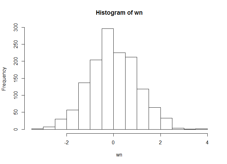
set.seed(1)
wn<-rnorm(1391)
hist(wn)
(2)
out<-data.frame(matrix(1:21,nrow=7,ncol=3))
for (i in 1:7) {
  tmp.p<-lm(msci.log[,i]~wn)
  tmp.p.beta<-tmp.p$coefficients[2]
  tmp.f.stat<-summary(tmp.p)$fstatistic
  tmp.p.p.value<-1-pf(tmp.f.stat["value"],tmp.f.stat["numdf"],tmp.f.stat["dendf"])
  tmp.p.adj.r.squared<-summary(tmp.p)$adj.r.squared
  out[i,]<-data.frame(matrix(c(tmp.p.beta, tmp.p.p.value, tmp.p.adj.r.squared), nrow=1))
}
colnames(out)<-c("推定値β^", "p値", "決定係数")
rownames(out)<-colnames(msci.log)
out
   推定値β^       p値    決定係数
ca  -0.005197388 0.5748192 -0.0004931680
fr  -0.003196312 0.6706261 -0.0005895938
ge  -0.003614680 0.6928374 -0.0006074941
it  -0.003411967 0.5995188 -0.0005212435
jp  -0.001184826 0.8467281 -0.0006930146
uk  -0.002621959 0.6630235 -0.0005831074
us  -0.002241276 0.5714044 -0.0004890948
調整済み決定係数なので、負の値になっているが実質ほぼ0。
(3)
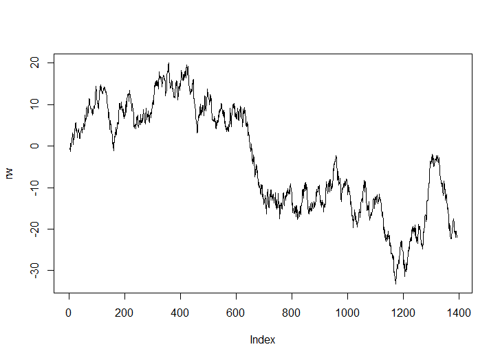
rw<-cumsum(wn)
plot(rw, type="l")
(4)
out<-data.frame(matrix(1:21,nrow=7,ncol=3))
for (i in 1:7) {
  tmp.p<-lm(msci.log[,i]~rw)
  tmp.p.beta<-tmp.p$coefficients[2]
  tmp.f.stat<-summary(tmp.p)$fstatistic
  tmp.p.p.value<-1-pf(tmp.f.stat["value"],tmp.f.stat["numdf"],tmp.f.stat["dendf"])
  tmp.p.adj.r.squared<-summary(tmp.p)$adj.r.squared
  out[i,]<-data.frame(matrix(c(tmp.p.beta, tmp.p.p.value, tmp.p.adj.r.squared), nrow=1))
}
colnames(out)<-c("推定値β^", "p値", "決定係数")
rownames(out)<-colnames(msci.log)
out
   推定値β^       p値    決定係数
ca -0.022671268   0        0.6988062
fr -0.017622486   0        0.6416288
ge -0.021094733   0        0.6201344
it -0.014705891   0        0.5976875
jp -0.013653738   0        0.5790067
uk -0.013868895   0        0.6199455
us -0.008966661   0        0.5982770
見せかけの回帰の現象が見られる。
テキストとホワイトノイズの値が異なるので値は一致しないが、p125の表6.1と同等にp値が0で決定係数が高めに出ている。
(5)
for (i in 1:1) {
  rw_1<-0
  y_1<-0
  rw_1[1]<-0
  y_1[1]<-0
  for (j in 2:1391) {
    rw_1[j]<-rw[j-1]
    y_1[j]<-msci.log[j-1,i]
  }
  tmp.p<-lm(msci.log[,i]~rw+rw_1+y_1)
  tmp.p.beta<-tmp.p$coefficients[2]
  tmp.f.stat<-summary(tmp.p)$fstatistic
  tmp.p.p.value<-1-pf(tmp.f.stat["value"],tmp.f.stat["numdf"],tmp.f.stat["dendf"])
  tmp.p.adj.r.squared<-summary(tmp.p)$adj.r.squared
  out[i,]<-data.frame(matrix(c(tmp.p.beta, tmp.p.p.value, tmp.p.adj.r.squared), nrow=1))
}
colnames(out)<-c("推定値β^", "p値", "決定係数")
rownames(out)<-colnames(msci.log)
out
   推定値β^       p値    決定係数
ca -0.007613280   0        0.8812688
fr -0.017622486   0        0.6416288
ge -0.021094733   0        0.6201344
it -0.014705891   0        0.5976875
jp -0.013653738   0        0.5790067
uk -0.013868895   0        0.6199455
us -0.008966661   0        0.5982770
見せかけの回帰の現象が見られる。
6.5
ppp<-read.table("ppp.txt", header=T)
(1)
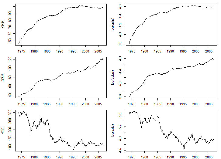
lcpijp<-ts(log(ppp$cpijp),start=c(1974,1),frequency=12)
lcpius<-ts(log(ppp$cpius),start=c(1974,1),frequency=12)
lexjp<-ts(log(ppp$exjp),start=c(1974,1),frequency=12)
par(mfrow=c(3,2))
par(mar=c(2,4,1,1))
ts.plot(ts(ppp$cpijp,start=c(1974,1),frequency=12),ylab="cpijp")
ts.plot(lcpijp,ylab="log(cpijp)")
ts.plot(ts(ppp$cpius,start=c(1974,1),frequency=12),ylab="cpius")
ts.plot(lcpius,ylab="log(cpius)")
ts.plot(ts(ppp$exjp,start=c(1974,1),frequency=12),ylab="exjp")
ts.plot(lexjp,ylab="log(exjp)")
(2)
library(tseries)
adf.test(lcpijp)
adf.test(lcpijp, alternative = "explosive")
adf.test(lcpius)
adf.test(lcpius, alternative = "explosive")
adf.test(lexjp)
adf.test(lexjp, alternative = "explosive")
> adf.test(lcpijp)

	Augmented Dickey-Fuller Test

data:  lcpijp
Dickey-Fuller = -4.0654, Lag order = 7, p-value = 0.01
alternative hypothesis: stationary

Warning message:
In adf.test(lcpijp) : p-value smaller than printed p-value
> adf.test(lcpijp, alternative = "explosive")

	Augmented Dickey-Fuller Test

data:  lcpijp
Dickey-Fuller = -4.0654, Lag order = 7, p-value = 0.99
alternative hypothesis: explosive

Warning message:
In adf.test(lcpijp, alternative = "explosive") :
  p-value smaller than printed p-value
> adf.test(lcpius)

	Augmented Dickey-Fuller Test

data:  lcpius
Dickey-Fuller = -2.4815, Lag order = 7, p-value =
0.3739
alternative hypothesis: stationary

> adf.test(lcpius, alternative = "explosive")

	Augmented Dickey-Fuller Test

data:  lcpius
Dickey-Fuller = -2.4815, Lag order = 7, p-value =
0.6261
alternative hypothesis: explosive

> adf.test(lexjp)

	Augmented Dickey-Fuller Test

data:  lexjp
Dickey-Fuller = -1.6156, Lag order = 7, p-value =
0.7396
alternative hypothesis: stationary

> adf.test(lexjp, alternative = "explosive")

	Augmented Dickey-Fuller Test

data:  lexjp
Dickey-Fuller = -1.6156, Lag order = 7, p-value =
0.2604
alternative hypothesis: explosive
(3)
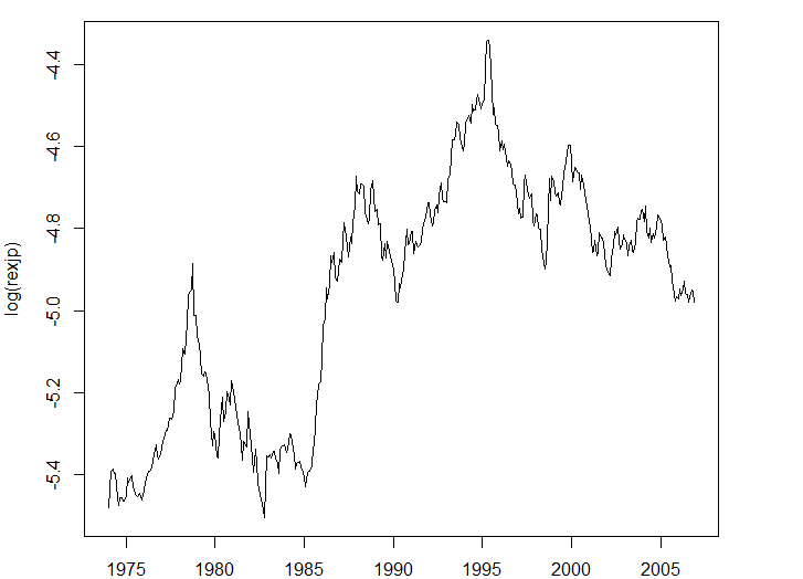
lrexjp<-lcpijp-lcpius-lexjp
par(mar=c(2,4,1,4))
plot(lrexjp, ylab="log(rexjp)")
(4)
PPP仮説は
$$
lcpijp \approx lexjp + lcpius
$$
であるから
$$
lcpijp - lcpius - lexjp = lrexjp \approx 0
$$
よりlrexjpが0に収束することを示唆している。
(5)
adf.test(lrexjp)
adf.test(lrexjp, alternative = "explosive")
adf.test(diff(lrexjp))
> adf.test(lrexjp)

	Augmented Dickey-Fuller Test

data:  lrexjp
Dickey-Fuller = -1.3335, Lag order = 7, p-value =
0.8587
alternative hypothesis: stationary

> adf.test(lrexjp, alternative = "explosive")

	Augmented Dickey-Fuller Test

data:  lrexjp
Dickey-Fuller = -1.3335, Lag order = 7, p-value =
0.1413
alternative hypothesis: explosive

> adf.test(diff(lrexjp))

	Augmented Dickey-Fuller Test

data:  diff(lrexjp)
Dickey-Fuller = -6.7109, Lag order = 7, p-value = 0.01
alternative hypothesis: stationary

Warning message:
In adf.test(diff(lrexjp)) : p-value smaller than printed p-value
より、単位根がある。このためlrexjpの値が収束しないので、PPP仮説を支持していない。
(6)
library(urca)
lrexjp.df<-data.frame(lcpijp, -lcpius, -lexjp)
lrexjp.vecm<-ca.jo(lrexjp.df, ecdet="none", type="eigen", K=6, spec="longrun", season=NULL)
summary(lrexjp.vecm)
> summary(lrexjp.vecm)

######################
# Johansen-Procedure #
######################

Test type: maximal eigenvalue statistic (lambda max) , with linear trend

Eigenvalues (lambda):
[1] 0.158408638 0.032735262 0.002925689

Values of teststatistic and critical values of test:

          test 10pct  5pct  1pct
r <= 2 |  1.14  6.50  8.18 11.65
r <= 1 | 12.98 12.91 14.90 19.19
r = 0  | 67.26 18.90 21.07 25.75

Eigenvectors, normalised to first column:
(These are the cointegration relations)

              lcpijp.l6 X.lcpius.l6 X.lexjp.l6
lcpijp.l6    1.00000000   1.0000000  1.0000000
X.lcpius.l6  0.02892562   0.2519313  0.7927706
X.lexjp.l6  -0.07537271  -0.3823289  0.1300192

Weights W:
(This is the loading matrix)

              lcpijp.l6 X.lcpius.l6    X.lexjp.l6
lcpijp.d   -0.021872635 0.002756738 -0.0007592322
X.lcpius.d  0.014398742 0.008619883 -0.0038549536
X.lexjp.d   0.002801142 0.061199460  0.0184638162
r = 1
r+1=2個の共和分関係が存在する。よってPPP仮説を支持する。
(7)
lcpica<-ts(log(ppp$cpica),start=c(1974,1),frequency=12)
lcpiuk<-ts(log(ppp$cpiuk),start=c(1974,1),frequency=12)
lexca<-ts(log(ppp$exca),start=c(1974,1),frequency=12)
lexuk<-ts(log(ppp$exuk),start=c(1974,1),frequency=12)

lrexca.df<-data.frame(lcpica, -lcpius, -lexca)
lrexca.vecm<-ca.jo(lrexca.df, ecdet="none", type="eigen", K=6, spec="longrun", season=NULL)
summary(lrexca.vecm)
######################
# Johansen-Procedure #
######################

Test type: maximal eigenvalue statistic (lambda max) , with linear trend

Eigenvalues (lambda):
[1] 0.104204155 0.016269511 0.002260424

Values of teststatistic and critical values of test:

          test 10pct  5pct  1pct
r <= 2 |  0.88  6.50  8.18 11.65
r <= 1 |  6.40 12.91 14.90 19.19
r = 0  | 42.92 18.90 21.07 25.75

Eigenvectors, normalised to first column:
(These are the cointegration relations)

             lcpica.l6 X.lcpius.l6 X.lexca.l6
lcpica.l6   1.00000000   1.0000000   1.000000
X.lcpius.l6 0.97756101   1.2966193   2.087184
X.lexca.l6  0.04893602   0.6192151  -1.629409

Weights W:
(This is the loading matrix)

              lcpica.l6  X.lcpius.l6    X.lexca.l6
lcpica.d   -0.013164472 -0.001479385  0.0003232371
X.lcpius.d  0.009339536 -0.007286482 -0.0011414028
X.lexca.d   0.032099791 -0.011930871  0.0031450132
lrexuk.df<-data.frame(lcpiuk, -lcpius, -lexuk)
lrexuk.vecm<-ca.jo(lrexuk.df, ecdet="none", type="eigen", K=6, spec="longrun", season=NULL)
summary(lrexuk.vecm)
######################
# Johansen-Procedure #
######################

Test type: maximal eigenvalue statistic (lambda max) , with linear trend

Eigenvalues (lambda):
[1] 0.128672334 0.030943227 0.007768275

Values of teststatistic and critical values of test:

          test 10pct  5pct  1pct
r <= 2 |  3.04  6.50  8.18 11.65
r <= 1 | 12.26 12.91 14.90 19.19
r = 0  | 53.72 18.90 21.07 25.75

Eigenvectors, normalised to first column:
(These are the cointegration relations)

             lcpiuk.l6 X.lcpius.l6 X.lexuk.l6
lcpiuk.l6    1.0000000   1.0000000   1.000000
X.lcpius.l6  0.5757486   1.3613908   1.945102
X.lexuk.l6  -2.0586854   0.9541808  -0.105148

Weights W:
(This is the loading matrix)

              lcpiuk.l6  X.lcpius.l6   X.lexuk.l6
lcpiuk.d   -0.005272950 -0.003607554  0.001152957
X.lcpius.d  0.002705188 -0.006229943 -0.003849241
X.lexuk.d   0.011352610 -0.017602665  0.026309049
r = 1
r+1=2個の共和分関係が存在する。よってPPP仮説を支持する。