Chatterjee順位相関というものですね。
この記事が話題ですが、もっと古くから(スライド資料時点で2013年)「21世紀の」相関と呼ばれるものがあります。
代表的な相関係数1
| 手法 | 特徴 | 備考 |
|---|---|---|
| ピアソンの積率相関係数2 | 2変数の線形な関係の強さを、共分散を標準偏差で割って無次元化して測る指標 | 一番スタンダードな相関係数 |
| スピアマンの順位相関係数3 | 順位に直した後の Pearson 相関 $\Rightarrow$ 順位の値(距離)まで使う(例:1位$\leftrightarrow$2位と1位$\leftrightarrow$100位は差が違う)。 | 外れ値に強いとされる相関係数(ケンドールよりは極端な順位に敏感) |
| ケンドールの順位相関係数4 | 2点の組$(i, j)$ を取ったとき、「順序が一致する確率 − 逆転する確率」 | 外れ値に強いとされる相関係数 |
| MIC(Maximal Information Coefficient 最大情報係数)5 | データをいろいろな格子(分割)で区切ったときの「相互情報量」を正規化して最大化し、線形に限らない幅広い関係性の強さを0〜1で測る指標 | 非線形に対応するが負の相関は表せない |
| HSIC test(Hilbert-Schmidt Independence Criterion test 再生核ヒルベルト空間を用いた独立性検定)6 7 | カーネルを使って2変数(または多変量)の独立性を検定し、「独立なら0に近い」統計量(HSIC)が十分大きいかで判断するテスト | 非線形に対応するが負の相関は表せない(理論上は0以上(ただし推定量はわずかに負になり得る)で上限なし)。p値での検定が主役 |
| Chatterjee順位相関8 | xを順位で並べたときにyがどれだけ一意に決まるか(予測できるか)を0〜1で測る、方向つき(x→y)の依存度指標 | 非線形に対応するが負の相関は表せない。$x\rightarrow y, y\rightarrow x$の依存度合いが異なれば値が異なる |
MICをイメージで言うと、
- x と yの散布図を格子で区切って、xの区画を知ると yの区画がどれだけ絞れるか(= 相互情報量がどれだけ大きいか)
- 区画が絞れればx, yに関係がある、つまり依存が強い
- 区画が絞れなければx, yに関係がない、つまり依存が弱い
HSIC test をイメージで言うと、
-
x と y をそれぞれ「似てる度」の表(類似度行列)に変換して、その2つの表が同じ並び方(同じ島・同じグループ構造)になっているかを見るテスト
- もし xで似てる2点が、yでも似てるなら $\rightarrow$ 2つの表が重なって依存してる(独立じゃない)
- もし xの似てる/似てないと yの似てる/似てないが無関係なら $\rightarrow$ 表はバラバラで 独立っぽい
-
「直線かどうか」じゃなくて、近いもの同士が近いままかを見てる、というイメージ
全体をまとめるとこう
- Pearson / Spearman / Kendall
- 「(線形 or 単調な)関係の向き(正/負)と強さ」を見る 符号つき相関
- MIC / HSIC / Chatterjee
- 「2変数が 独立かどうか(=何らかの依存があるか)」という観点で見る(符号は基本出ない)
- HSICは「検定」(p値で独立を棄却するか)
- MIC / Chatterjeeは「依存度スコア」(0〜1で強さ)で、必要ならp値を付けられる実装もある
- Chatterjee順位相関はxとyの依存の向きも見られるが、因果関係を意味しない(交絡がある場合などを考慮していない)
- 「2変数が 独立かどうか(=何らかの依存があるか)」という観点で見る(符号は基本出ない)
使い分け例
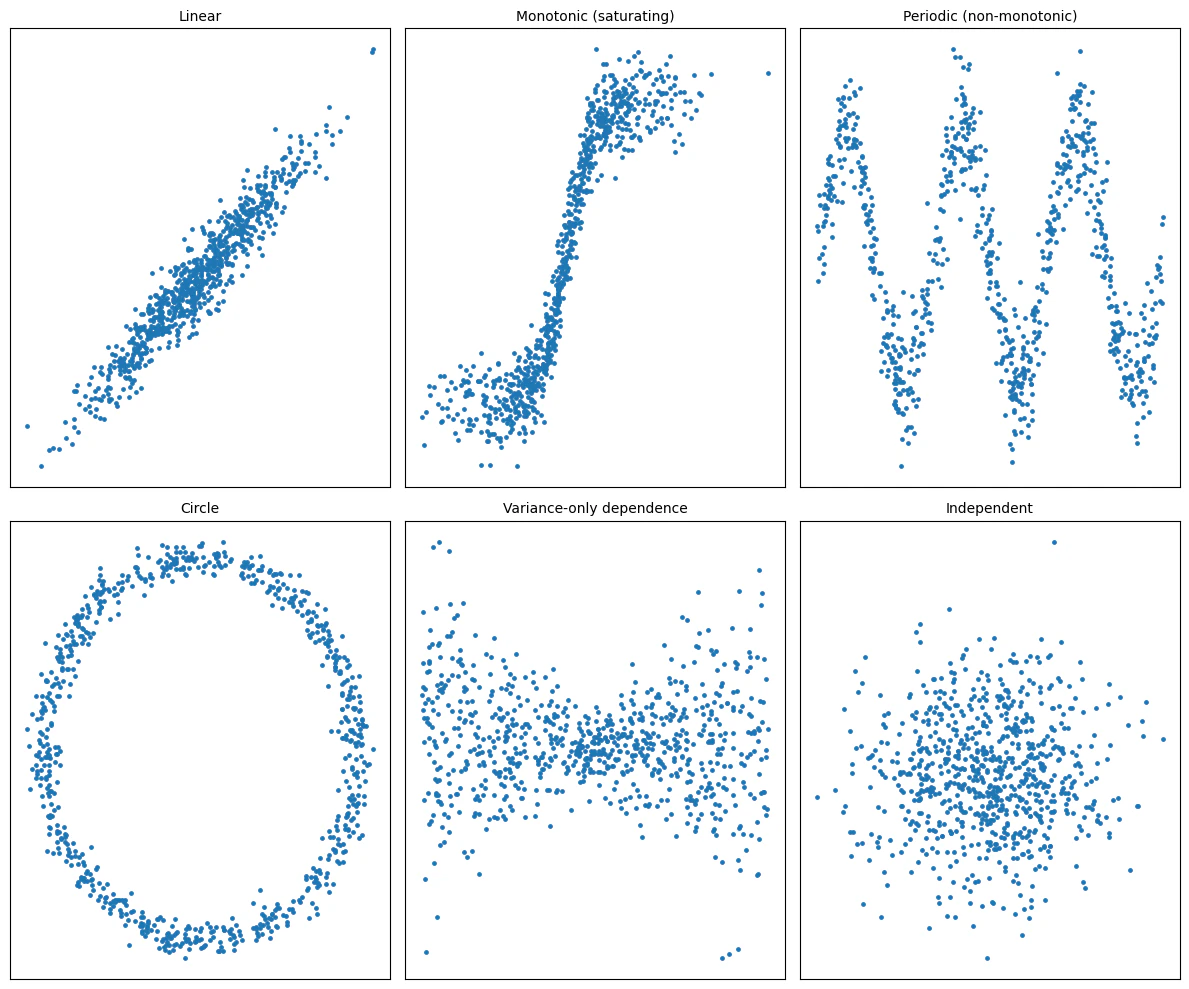
どのような挙動かサンプルデータでテスト
- MICをそのまま計算するには MINE(MIC)実装が必要(例:minepy等)。今回は環境都合で MIC(simple) を使ってます。ごめんなさい
- MIC(simple) は MINEのMICと一致する保証はなく、挙動の雰囲気確認用です
各統計量と(p値)
| case | Pearson r | Spearman rho | Kendall tau | MIC (simple) | HSIC | Chatterjee ξ(x->y) | Chatterjee ξ(y->x) |
|---|---|---|---|---|---|---|---|
| Linear(Pearsonが強い) | 0.956(0.0) | 0.950(0.0) | 0.813 | 0.675 | 0.692(1.05E-122) | 0.725(3.22E-231) | 0.712(6.86E-223) |
| Monotonic(順位系が強い) | 0.897(6.42E-286) | 0.952(0.0) | 0.808 | 0.917 | 0.829(2.20E-146) | 0.744(6.42E-243) | 0.740(2.64E-240) |
| Periodic(非線形指標が強い) | -0.197(2.00E-08) | -0.198(1.57E-08) | -0.134 | 0.710 | 0.018(8.95E-05) | 0.675(1.77E-200) | 0.061(0.003) |
| Circle(Pearson≈0でも依存は強い) | -0.011(0.753) | -0.010(0.788) | -0.009 | 0.489 | 0.070(5.31E-14) | 0.203(5.71E-20) | 0.173(4.46E-15) |
| Variance-only dependence 分散がxに依存(平均は0) | -0.092(0.009) | -0.080(0.024) | -0.053 | 0.120 | 0.042(4.79E-09) | 0.002(0.460) | 0.008(0.361) |
| Independent(全部小さい) | 0.013(0.718) | -0.003(0.929) | -0.003 | 0.089 | -0.001(1.0) | 0.005(0.419) | -0.017(0.781) |
- 注:
- p値は「強さ」ではなく「独立からのズレの確からしさ」なので、係数(効果量)とセットで見る
- Kendall tauはp値略
- MIC(simple)は簡易版のためp値はなし
- HSIC stat はスケール依存。p値が主
- Linear
- Pearsonが強く、Spearmanも同等
- MIC、HSIC、Chatterjeeでも依存を捉えている
- Monotonic
- Spearmanが強く、Pearsonはやや落ちる
- MIC、HSIC、Chatterjeeでも依存を捉えている
- Periodic
- Pearson、Spearmanでは厳しいがp値は小さく出ている
- MICは依存を捉えている
- HSICは依存を検出
- Chatterjeeではx→y が大きく、y→x は小さい(方向が出る)
- Circle
- Pearson、Spearmanでは無相関反応
- MICはまずまず依存を捉えている
- HSICは依存を検出
- Chatterjeeでは両方向とも中程度で、方向差は小さい
- Variance-only dependence
- Pearson、Spearmanでは弱い(ほぼ0)
- MICではごく弱い依存
- HSICでは依存を検出
- Chatterjeeではほぼ依存がない
- Independent
- 全てで無相関反応(独立と考えられる)
(今回はKendall特有のサンプルがなく、Spearmanに準じている)
実装例
- 環境
- Google Colaboratory
- コード生成
- ChatGPT 5.2 思考 思考の拡張
pip -q install -U "scipy>=1.15" numpy pandas matplotlib hyppo
import numpy as np
import pandas as pd
import matplotlib.pyplot as plt

from scipy.stats import pearsonr, spearmanr, kendalltau, chatterjeexi
from hyppo.independence import Hsic

# -----------------------------
# 簡易MIC(デモ用)
# - quantile binning + grid search
# - MIを log(min(bins)) で正規化して最大値を取る
# -----------------------------
def mic_simple(x, y, max_bins=20, eps=1e-12):
    x = np.asarray(x).ravel()
    y = np.asarray(y).ravel()
    n = x.size
    best = 0.0

    for bx in range(2, max_bins + 1):
        ex = np.unique(np.quantile(x, np.linspace(0, 1, bx + 1)))
        if ex.size < 3:
            continue

        for by in range(2, max_bins + 1):
            ey = np.unique(np.quantile(y, np.linspace(0, 1, by + 1)))
            if ey.size < 3:
                continue

            # joint histogram (stable & shape-safe)
            counts, _, _ = np.histogram2d(x, y, bins=[ex, ey])
            pxy = counts / n
            px = pxy.sum(axis=1, keepdims=True)          # (hx,1)
            py = pxy.sum(axis=0, keepdims=True)          # (1,hy)
            denom = px * py                               # (hx,hy)

            nz = pxy > 0
            mi = np.sum(pxy[nz] * np.log((pxy[nz] + eps) / (denom[nz] + eps)))

            norm = np.log(min(pxy.shape))
            if norm > 0:
                mic = mi / norm
                if mic > best:
                    best = mic

    return float(np.clip(best, 0.0, 1.0))


# -----------------------------
# “違いが見える”データ
# -----------------------------
def make_cases(seed=12345, n=800):
    rng = np.random.default_rng(seed)
    cases = []

    # 線形:Pearsonが強い
    x = rng.normal(size=n)
    y = 2.0 * x + rng.normal(scale=0.6, size=n)
    cases.append(("Linear", x, y, "直線関係(Pearsonが強い)"))

    # 単調だが飽和:Spearmanが強い
    x = rng.normal(size=n)
    y = np.tanh(2.0 * x) + rng.normal(scale=0.15, size=n)
    cases.append(("Monotonic (saturating)", x, y, "単調だが飽和(順位系が強い)"))

    # 周期・非単調:Pearson/Spearmanが落ち、HSIC/MIC/xiが拾いやすい
    x = rng.uniform(0, 1, size=n)
    y = np.sin(6 * np.pi * x) + rng.normal(scale=0.25, size=n)
    cases.append(("Periodic (non-monotonic)", x, y, "周期・非単調(非線形指標が強い)"))

    # 円:相関0でも依存は強い
    t = rng.uniform(0, 2*np.pi, size=n)
    x = np.cos(t) + rng.normal(scale=0.05, size=n)
    y = np.sin(t) + rng.normal(scale=0.05, size=n)
    cases.append(("Circle", x, y, "円(Pearson≈0でも依存は強い)"))

    # 分散だけ依存(平均は0)
    x = rng.uniform(-1, 1, size=n)
    y = rng.normal(loc=0.0, scale=0.3 + 1.2*np.abs(x), size=n)
    cases.append(("Variance-only dependence", x, y, "分散がxに依存(平均は0)"))

    # 独立
    x = rng.normal(size=n)
    y = rng.normal(size=n)
    cases.append(("Independent", x, y, "独立(全部小さい)"))

    return cases


def compute_metrics(cases, seed=12345, mic_bins=20):
    hsic = Hsic()
    rows = []
    for name, x, y, note in cases:
        x = np.asarray(x).ravel()
        y = np.asarray(y).ravel()

        r, p_r = pearsonr(x, y)
        rho, p_rho = spearmanr(x, y)

        tau, p_tau = kendalltau(x, y)

        # HSIC(独立性検定)
        hs_stat, hs_p = hsic.test(
            x.reshape(-1, 1), y.reshape(-1, 1),
            random_state=seed
        )

        # Chatterjee順位相関 xi(方向あり)
        xi_xy = chatterjeexi(x, y, y_continuous=True, method="asymptotic")
        xi_yx = chatterjeexi(y, x, y_continuous=True, method="asymptotic")

        # MIC(簡易)
        mic = mic_simple(x, y, max_bins=mic_bins)

        rows.append({
            "case": name,
            "note": note,
            "Pearson r": r, "Pearson p": p_r,
            "Spearman rho": rho, "Spearman p": p_rho,
            "Kendall tau": tau, "Kendall p": p_tau,
            "MIC (simple)": mic,
            "HSIC stat": hs_stat, "HSIC p": hs_p,
            "xi(x->y)": xi_xy.statistic, "xi p(x->y)": xi_xy.pvalue,
            "xi(y->x)": xi_yx.statistic, "xi p(y->x)": xi_yx.pvalue,
        })

    return pd.DataFrame(rows)


# -----------------------------
# 実行
# -----------------------------
cases = make_cases(seed=12345, n=800)

df = compute_metrics(cases, seed=12345, mic_bins=20)

pd.set_option("display.precision", 4)
display(df[[
    "case","note",
    "Pearson r","Spearman rho","Kendall tau","MIC (simple)","HSIC stat","xi(x->y)","xi(y->x)",
    "Pearson p","Spearman p","Kendall p","HSIC p","xi p(x->y)","xi p(y->x)"
]])


# 散布図で形も確認
cols = 3
rows = int(np.ceil(len(cases) / cols))
plt.figure(figsize=(12, 10))
for i, (name, x, y, note) in enumerate(cases, 1):
    ax = plt.subplot(rows, cols, i)
    ax.scatter(x, y, s=6)
    ax.set_title(name, fontsize=10)
    ax.set_xticks([]); ax.set_yticks([])
plt.tight_layout()
plt.show()
- 注:
- HSICのp値は chi2_approx(χ²近似)
- Chatterjee ξのp値は method='asymptotic'(漸近近似)
- II部:知っていると得 1. MIC vs HSIC:直線でなくとも相関はある⁉️
のUpdate記事です。
-
その他にもいろいろ実はあります。c.f. Wikipedia: 相関係数 ↩
-
PEARSON, Karl. VII. Note on regression and inheritance in the case of two parents. proceedings of the royal society of London, 1895, 58.347-352: 240-242. https://www.jstor.org/stable/115794 ↩
-
SPEARMAN, Charles. The proof and measurement of association between two things. 1904. https://www.jstor.org/stable/1412159 (引用者注:1904年のはずがGoogle Scholarの被引用情報だと1961になっています) ↩
-
KENDALL, Maurice G. A new measure of rank correlation. Biometrika, 1938, 30.1-2: 81-93. https://academic.oup.com/biomet/article-abstract/30/1-2/81/176907 ↩
-
RESHEF, David N., et al. Detecting novel associations in large data sets. science, 2011, 334.6062: 1518-1524. https://www.science.org/doi/10.1126/science.1205438 ↩
-
GRETTON, Arthur, et al. Measuring statistical dependence with Hilbert-Schmidt norms. In: International conference on algorithmic learning theory. Berlin, Heidelberg: Springer Berlin Heidelberg, 2005. p. 63-77. https://www.gatsby.ucl.ac.uk/~gretton/papers/GreBouSmoSch05.pdf ↩
-
GRETTON, Arthur. A simpler condition for consistency of a kernel independence test. arXiv preprint arXiv:1501.06103, 2015. https://arxiv.org/abs/1501.06103 ↩
-
CHATTERJEE, Sourav. A new coefficient of correlation. Journal of the American Statistical Association, 2021, 116.536: 2009-2022. https://www.tandfonline.com/doi/full/10.1080/01621459.2020.1758115 ↩