『経済・ファイナンスデータの計量時系列分析』
の章末問題で「コンピュータを用いて」とあるものをRで解いています。

7.4
(1)
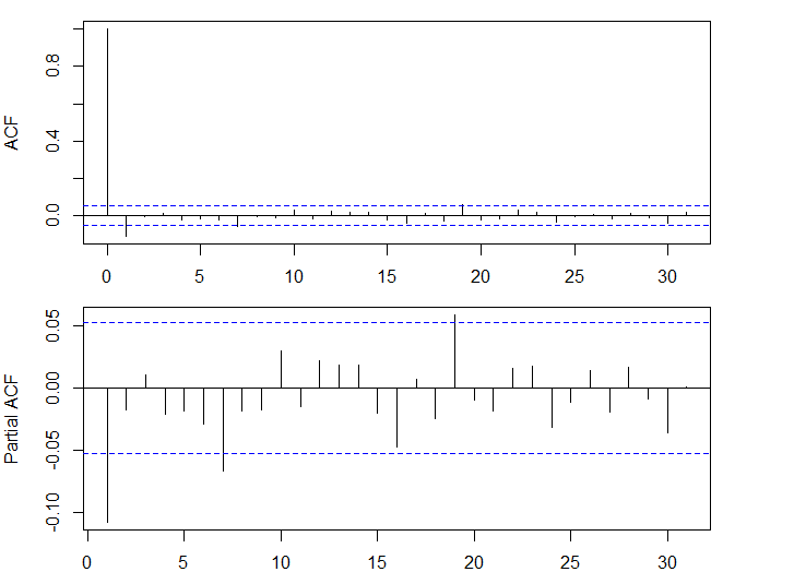
- 大きな自己相関はみられない
msci_day<-read.table("msci_day.txt",header=T)
par(mfrow=c(2,1))
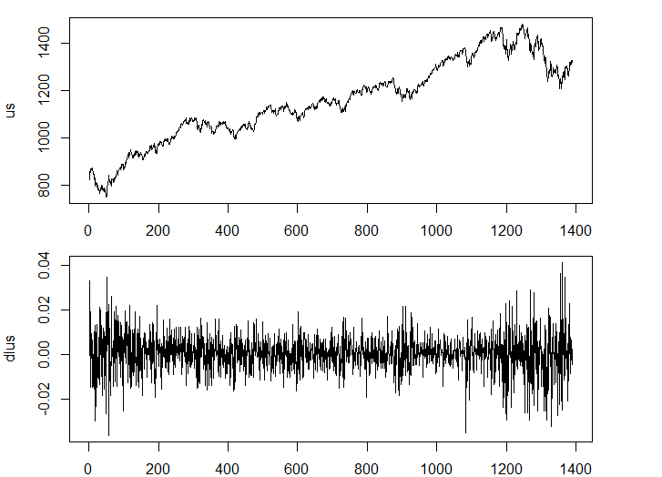
us<-msci_day$us
plot(us, type="l")
dlus<-diff(log(us))
plot(dlus, type="l")
acf(dlus)
pacf(dlus)
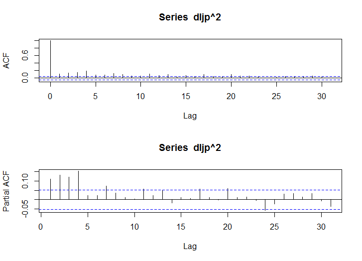
(2)
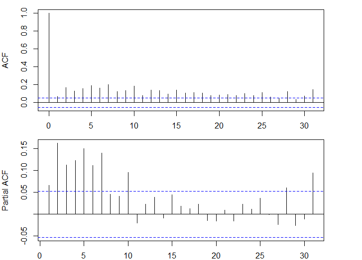
- 大きな自己相関がみられる
acf(dlus^2)
pacf(dlus^2)
(3)
# fGarch
library(fGarch)

dlus.garch<-garchFit(formula=~arma(1,0)+garch(1,1), data=dlus, trace=F)
summary(dlus.garch)
Title:
 GARCH Modelling

Call:
 garchFit(formula = ~arma(1, 0) + garch(1, 1), data = dlus, trace = F)

Mean and Variance Equation:
 data ~ arma(1, 0) + garch(1, 1)
<environment: 0x0000000015605008>
 [data = dlus]

Conditional Distribution:
 norm

Coefficient(s):
         mu          ar1        omega       alpha1
 4.6782e-04  -7.8543e-02   1.0128e-06   5.0598e-02
      beta1
 9.3444e-01

Std. Errors:
 based on Hessian

Error Analysis:
         Estimate  Std. Error  t value Pr(>|t|)
mu      4.678e-04   1.961e-04    2.386  0.01704 *
ar1    -7.854e-02   2.795e-02   -2.810  0.00495 **
omega   1.013e-06   3.489e-07    2.903  0.00370 **
alpha1  5.060e-02   9.937e-03    5.092 3.55e-07 ***
beta1   9.344e-01   1.314e-02   71.103  < 2e-16 ***
---
Signif. codes:  0 ‘***’ 0.001 ‘**’ 0.01 ‘*’ 0.05 ‘.’ 0.1 ‘ ’ 1

Log Likelihood:
 4756.516    normalized:  3.421954

Description:
 Sun Jan 29 10:00:51 2017 by user: aoki


Standardised Residuals Tests:
                                Statistic p-Value
 Jarque-Bera Test   R    Chi^2  180.9516  0
 Shapiro-Wilk Test  R    W      0.9840602 2.999756e-11
 Ljung-Box Test     R    Q(10)  10.05805  0.4354152
 Ljung-Box Test     R    Q(15)  14.6652   0.4757913
 Ljung-Box Test     R    Q(20)  17.64631  0.6106947
 Ljung-Box Test     R^2  Q(10)  13.96237  0.174715
 Ljung-Box Test     R^2  Q(15)  16.33594  0.3600828
 Ljung-Box Test     R^2  Q(20)  17.08671  0.6473361
 LM Arch Test       R    TR^2   15.48142  0.2161583

Information Criterion Statistics:
      AIC       BIC       SIC      HQIC
-6.836714 -6.817875 -6.836740 -6.829669
# rugarch
library(rugarch)

dlus.spec<-ugarchspec(variance.model=list(model="sGARCH", garchOrder=c(1,1)), mean.model=list(armaOrder=c(1,0), include.mean=T))
dlus.garch<-ugarchfit(data=dlus, spec=dlus.spec)
dlus.garch
> dlus.garch

*---------------------------------*
*          GARCH Model Fit        *
*---------------------------------*

Conditional Variance Dynamics
-----------------------------------
GARCH Model	: sGARCH(1,1)
Mean Model	: ARFIMA(1,0,0)
Distribution	: norm

Optimal Parameters
------------------------------------
        Estimate  Std. Error  t value Pr(>|t|)
mu      0.000441    0.000183  2.41849 0.015585
ar1    -0.079111    0.028059 -2.81940 0.004811
omega   0.000001    0.000002  0.59728 0.550317
alpha1  0.049525    0.020256  2.44490 0.014489
beta1   0.935539    0.023125 40.45591 0.000000

Robust Standard Errors:
        Estimate  Std. Error   t value Pr(>|t|)
mu      0.000441    0.000355  1.243796 0.213575
ar1    -0.079111    0.027009 -2.929059 0.003400
omega   0.000001    0.000030  0.032807 0.973829
alpha1  0.049525    0.330906  0.149664 0.881029
beta1   0.935539    0.390027  2.398653 0.016455

LogLikelihood : 4751.628

*---------------------------------*
*          GARCH Model Fit        *
*---------------------------------*

Conditional Variance Dynamics
-----------------------------------
GARCH Model	: sGARCH(1,1)
Mean Model	: ARFIMA(1,0,0)
Distribution	: norm

Optimal Parameters
------------------------------------
        Estimate  Std. Error  t value Pr(>|t|)
mu      0.000441    0.000183  2.41849 0.015585
ar1    -0.079111    0.028059 -2.81940 0.004811
omega   0.000001    0.000002  0.59728 0.550317
alpha1  0.049525    0.020256  2.44490 0.014489
beta1   0.935539    0.023125 40.45591 0.000000

Robust Standard Errors:
        Estimate  Std. Error   t value Pr(>|t|)
mu      0.000441    0.000355  1.243796 0.213575
ar1    -0.079111    0.027009 -2.929059 0.003400
omega   0.000001    0.000030  0.032807 0.973829
alpha1  0.049525    0.330906  0.149664 0.881029
beta1   0.935539    0.390027  2.398653 0.016455

LogLikelihood : 4751.628

Information Criteria
------------------------------------

Akaike       -6.8297
Bayes        -6.8108
Shibata      -6.8297
Hannan-Quinn -6.8226

Weighted Ljung-Box Test on Standardized Residuals
------------------------------------
                        statistic p-value
Lag[1]                   0.001242  0.9719
Lag[2*(p+q)+(p+q)-1][2]  0.385088  0.9856
Lag[4*(p+q)+(p+q)-1][5]  1.217200  0.9092
d.o.f=1
H0 : No serial correlation

Weighted Ljung-Box Test on Standardized Squared Residuals
------------------------------------
                        statistic p-value
Lag[1]                      3.730 0.05345
Lag[2*(p+q)+(p+q)-1][5]     4.288 0.22027
Lag[4*(p+q)+(p+q)-1][9]     4.932 0.43945
d.o.f=2

Weighted ARCH LM Tests
------------------------------------
            Statistic Shape Scale P-Value
ARCH Lag[3]   0.02518 0.500 2.000  0.8739
ARCH Lag[5]   1.14491 1.440 1.667  0.6905
ARCH Lag[7]   1.28023 2.315 1.543  0.8642
            Statistic Shape Scale P-Value
ARCH Lag[3]   0.02518 0.500 2.000  0.8739
ARCH Lag[5]   1.14491 1.440 1.667  0.6905
ARCH Lag[7]   1.28023 2.315 1.543  0.8642

Nyblom stability test
------------------------------------
Joint Statistic:  162.9923
Individual Statistics:
mu      0.04725
ar1     0.15181
omega  16.76474
alpha1  0.32187
beta1   0.21276

Asymptotic Critical Values (10% 5% 1%)
Joint Statistic:     	 1.28 1.47 1.88
Individual Statistic:	 0.35 0.47 0.75

Sign Bias Test
------------------------------------
                   t-value    prob sig
Sign Bias            1.097 0.27267
Negative Sign Bias   1.033 0.30178
Positive Sign Bias   1.795 0.07293   *
Joint Effect         8.666 0.03408  **


Adjusted Pearson Goodness-of-Fit Test:
------------------------------------
  group statistic p-value(g-1)
1    20     88.73    5.556e-11
2    30    113.06    7.184e-12
3    40    110.26    1.005e-08
4    50    140.36    9.542e-11


Elapsed time : 1.15019
-
fGarch
mu = 4.678e-04
ar1 =-7.854e-02
omega = 1.013e-06
alpha1= 5.060e-02
beta1 = 9.344e-01 -
rugarch
mu = 0.000441
ar1 =-0.079111
omega = 0.000001
alpha1= 0.049525
beta1 = 0.935539
(4)
dlus.spec<-ugarchspec(variance.model=list(model="gjrGARCH", garchOrder=c(1,1)), mean.model=list(armaOrder=c(1,0), include.mean=T))
dlus.gjr<-ugarchfit(data=dlus, spec=dlus.spec)
dlus.gjr
> dlus.gjr<-ugarchfit(data=dlus, spec=dlus.spec)
> dlus.gjr

*---------------------------------*
*          GARCH Model Fit        *
*---------------------------------*

Conditional Variance Dynamics
-----------------------------------
GARCH Model	: gjrGARCH(1,1)
Mean Model	: ARFIMA(1,0,0)
Distribution	: norm

Optimal Parameters
------------------------------------
        Estimate  Std. Error   t value Pr(>|t|)
mu      0.000245    0.000183  1.340180 0.180187
ar1    -0.074942    0.027716 -2.703945 0.006852
omega   0.000001    0.000001  0.879222 0.379281
alpha1  0.000000    0.009631  0.000018 0.999986
beta1   0.943001    0.013853 68.069707 0.000000
gamma1  0.082897    0.019106  4.338717 0.000014

Robust Standard Errors:
        Estimate  Std. Error   t value Pr(>|t|)
mu      0.000245    0.000157  1.559756 0.118818
ar1    -0.074942    0.023622 -3.172597 0.001511
omega   0.000001    0.000015  0.063334 0.949501
alpha1  0.000000    0.048887  0.000004 0.999997
beta1   0.943001    0.155045  6.082123 0.000000
gamma1  0.082897    0.149275  0.555334 0.578666

LogLikelihood : 4768.721

Information Criteria
------------------------------------

Akaike       -6.8528
Bayes        -6.8302
Shibata      -6.8529
Hannan-Quinn -6.8444

Weighted Ljung-Box Test on Standardized Residuals
------------------------------------
                        statistic p-value
Lag[1]                   0.003938  0.9500
Lag[2*(p+q)+(p+q)-1][2]  0.453423  0.9744
Lag[4*(p+q)+(p+q)-1][5]  1.435205  0.8622
d.o.f=1
H0 : No serial correlation

Weighted Ljung-Box Test on Standardized Squared Residuals
------------------------------------
                        statistic p-value
Lag[1]                      4.918 0.02658
Lag[2*(p+q)+(p+q)-1][5]     5.404 0.12381
Lag[4*(p+q)+(p+q)-1][9]     6.045 0.29308
d.o.f=2

Weighted ARCH LM Tests
------------------------------------
                        statistic p-value
Lag[1]                   0.003938  0.9500
Lag[2*(p+q)+(p+q)-1][2]  0.453423  0.9744
Lag[4*(p+q)+(p+q)-1][5]  1.435205  0.8622
d.o.f=1
H0 : No serial correlation

Weighted Ljung-Box Test on Standardized Squared Residuals
------------------------------------
                        statistic p-value
Lag[1]                      4.918 0.02658
Lag[2*(p+q)+(p+q)-1][5]     5.404 0.12381
Lag[4*(p+q)+(p+q)-1][9]     6.045 0.29308
d.o.f=2

Weighted ARCH LM Tests
------------------------------------
            Statistic Shape Scale P-Value
ARCH Lag[3]    0.4768 0.500 2.000  0.4899
ARCH Lag[5]    0.9559 1.440 1.667  0.7461
ARCH Lag[7]    1.1364 2.315 1.543  0.8904

Nyblom stability test
------------------------------------
Joint Statistic:  122.7693
Individual Statistics:
mu      0.1306
ar1     0.1738
omega  12.7333
alpha1  0.3491
beta1   0.1656
gamma1  0.2125

Asymptotic Critical Values (10% 5% 1%)
Joint Statistic:     	 1.49 1.68 2.12
Individual Statistic:	 0.35 0.47 0.75

Sign Bias Test
------------------------------------
                   t-value    prob sig
Sign Bias            1.559 0.11925
Negative Sign Bias   1.936 0.05303   *
Positive Sign Bias   1.467 0.14253
Joint Effect         9.124 0.02769  **


Adjusted Pearson Goodness-of-Fit Test:
------------------------------------
  group statistic p-value(g-1)
1    20     77.88    4.293e-09
2    30     86.60    1.202e-07
3    40    100.36    2.610e-07
4    50    103.09    1.006e-05


Elapsed time : 1.177835
out<-data.frame()
omega<-1e-6
alpha<-1e-6
beta<-0.943001
gamma<-0.082897
ht<-seq(1,3)
for (ht1 in c(0.5,1,2)) {
  i<-1
  for (ut1 in -2:2) {
    ht[i]<-omega+beta*ht1+alpha*ut1^2+gamma*ut1^2*sign(ut1<0)
    i<-i+1
  }
  out<-rbind(out, ht)
}
names(out)<-c(-2, -1, 0, 1, 2)
row.names(out)<-c(0.5, 1, 2)
out
           -2        -1         0         1         2
0.5 0.8030935 0.5543995 0.4715015 0.4715025 0.4715055
1   1.2745940 1.0259000 0.9430020 0.9430030 0.9430060
2   2.2175950 1.9689010 1.8860030 1.8860040 1.8860070
レバレッジ効果がある
(5)
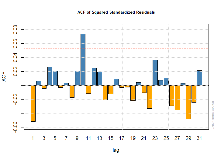
- 11を選択
plot(dlus.garch)
plot(dlus.gjr)
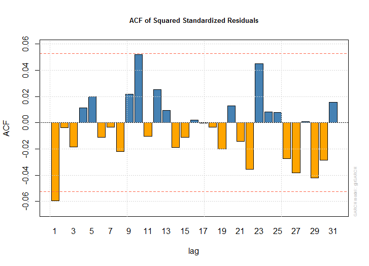
(6)
dlus.spec<-ugarchspec(variance.model=list(model="eGARCH", garchOrder=c(1,1)), mean.model=list(armaOrder=c(1,0), include.mean=T))
dlus.egarch<-ugarchfit(data=dlus, spec=dlus.spec)
dlus.egarch
*---------------------------------*
*          GARCH Model Fit        *
*---------------------------------*

Conditional Variance Dynamics
-----------------------------------
GARCH Model	: eGARCH(1,1)
Mean Model	: ARFIMA(1,0,0)
Distribution	: norm

Optimal Parameters
------------------------------------
        Estimate  Std. Error    t value Pr(>|t|)
mu      0.000277    0.000195     1.4201 0.155567
ar1    -0.081870    0.032705    -2.5033 0.012304
omega  -0.166643    0.002957   -56.3473 0.000000
alpha1 -0.087830    0.012714    -6.9080 0.000000
beta1   0.982551    0.000020 48090.9514 0.000000
gamma1  0.078968    0.000391   202.0952 0.000000

Robust Standard Errors:
        Estimate  Std. Error    t value Pr(>|t|)
mu      0.000277    0.000214     1.2924 0.196233
ar1    -0.081870    0.034178    -2.3954 0.016601
omega  -0.166643    0.003663   -45.4988 0.000000
alpha1 -0.087830    0.012832    -6.8448 0.000000
beta1   0.982551    0.000024 40637.8939 0.000000
gamma1  0.078968    0.000521   151.5471 0.000000

LogLikelihood : 4767.201

Information Criteria
------------------------------------

Akaike       -6.8506
Bayes        -6.8280
Shibata      -6.8507
Hannan-Quinn -6.8422

Weighted Ljung-Box Test on Standardized Residuals
------------------------------------
                        statistic p-value
Lag[1]                   0.005655  0.9401
Lag[2*(p+q)+(p+q)-1][2]  0.504447  0.9632
Lag[4*(p+q)+(p+q)-1][5]  1.590462  0.8240
d.o.f=1
H0 : No serial correlation

Weighted Ljung-Box Test on Standardized Squared Residuals
------------------------------------
                        statistic p-value
Lag[1]                      4.386 0.03624
Lag[2*(p+q)+(p+q)-1][5]     4.918 0.15978
Lag[4*(p+q)+(p+q)-1][9]     5.652 0.34020
d.o.f=2

Weighted ARCH LM Tests
------------------------------------
            Statistic Shape Scale P-Value
ARCH Lag[3]   0.07761 0.500 2.000  0.7806
ARCH Lag[5]   1.23064 1.440 1.667  0.6659
ARCH Lag[7]   1.39694 2.315 1.543  0.8418

Nyblom stability test
------------------------------------
Joint Statistic:  2.5097
Individual Statistics:
mu     0.2007
ar1    0.1198
omega  0.2873
alpha1 1.2433
beta1  0.2688
gamma1 0.2354

Asymptotic Critical Values (10% 5% 1%)
Joint Statistic:     	 1.49 1.68 2.12
Individual Statistic:	 0.35 0.47 0.75

Sign Bias Test
------------------------------------
                   t-value    prob sig
Sign Bias            1.441 0.14975
Negative Sign Bias   1.967 0.04941  **
Positive Sign Bias   1.387 0.16578
Joint Effect         8.142 0.04317  **


Adjusted Pearson Goodness-of-Fit Test:
------------------------------------
  group statistic p-value(g-1)
1    20     74.78    1.452e-08
2    30     83.45    3.577e-07
3    40     87.99    1.202e-05
4    50    119.64    7.685e-08


Elapsed time : 0.8469431
out<-data.frame()
omega<--0.166646
alpha<--0.087830
beta<-0.982551
gamma<-0.078968
ht<-seq(1,3)
for (ht1 in c(0.5,1,2)) {
  i<-1
  for (ut1 in -2:2) {
    ht[i]<-omega+beta*ht1+alpha*ut1^2+gamma*ut1^2*sign(ut1<0)
    i<-i+1
  }
  out<-rbind(out, ht)
}
names(out)<-c(-2, -1, 0, 1, 2)
row.names(out)<-c(0.5, 1, 2)
out
              -2        -1         0         1          2
0.5 0.2891845 0.3157705 0.3246325 0.2368025 -0.0266875
1   0.7804600 0.8070460 0.8159080 0.7280780  0.4645880
2   1.7630110 1.7895970 1.7984590 1.7106290  1.4471390
        -2        -1         0         1          2
0.5 0.2891845 0.3157705 0.3246325 0.2368025 -0.0266875
1   0.7804600 0.8070460 0.8159080 0.7280780  0.4645880
2   1.7630110 1.7895970 1.7984590 1.7106290  1.4471390
レバレッジ効果がある
(7)
- 11を選択
plot(dlus.egarch)
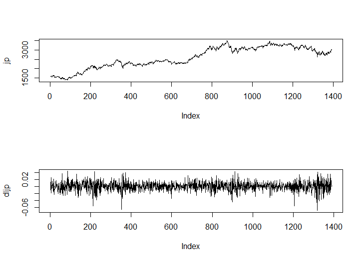
(8)
par(mfrow=c(2,1))
jp<-msci_day$jp
plot(jp, type="l")
dljp<-diff(log(jp))
plot(dljp, type="l")
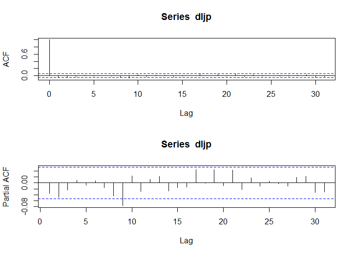
acf(dljp)
pacf(dljp)
acf(dljp^2)
pacf(dljp^2)
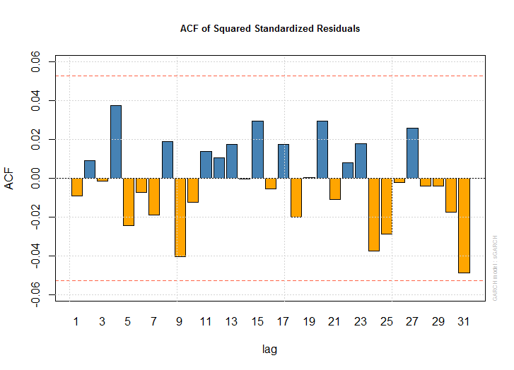
# GARCH
dljp.spec<-ugarchspec(variance.model=list(model="sGARCH", garchOrder=c(1,1)), mean.model=list(armaOrder=c(1,0), include.mean=T))
dljp.garch<-ugarchfit(data=dljp, spec=dljp.spec)
dljp.garch
*---------------------------------*
*          GARCH Model Fit        *
*---------------------------------*

Conditional Variance Dynamics
-----------------------------------
GARCH Model	: sGARCH(1,1)
Mean Model	: ARFIMA(1,0,0)
Distribution	: norm

Optimal Parameters
------------------------------------
        Estimate  Std. Error  t value Pr(>|t|)
mu      0.000566    0.000298  1.90212 0.057156
ar1    -0.010948    0.028309 -0.38675 0.698944
omega   0.000005    0.000003  1.39533 0.162918
alpha1  0.083277    0.003737 22.28493 0.000000
beta1   0.889458    0.011228 79.22073 0.000000

Robust Standard Errors:
        Estimate  Std. Error  t value Pr(>|t|)
mu      0.000566    0.000282  2.00790 0.044653
ar1    -0.010948    0.025292 -0.43289 0.665098
omega   0.000005    0.000011  0.43276 0.665188
alpha1  0.083277    0.040851  2.03853 0.041497
beta1   0.889458    0.027516 32.32567 0.000000

LogLikelihood : 4150.981

Information Criteria
------------------------------------

Akaike       -5.9654
Bayes        -5.9466
Shibata      -5.9655
Hannan-Quinn -5.9584

Weighted Ljung-Box Test on Standardized Residuals
------------------------------------
                        statistic p-value
Lag[1]                    0.02266  0.8803
Lag[2*(p+q)+(p+q)-1][2]   1.08159  0.6901
Lag[4*(p+q)+(p+q)-1][5]   1.86771  0.7491
d.o.f=1
H0 : No serial correlation

Weighted Ljung-Box Test on Standardized Squared Residuals
------------------------------------
                        statistic p-value
Lag[1]                     0.1186  0.7306
Lag[2*(p+q)+(p+q)-1][5]    1.1543  0.8239
Lag[4*(p+q)+(p+q)-1][9]    2.5367  0.8323
d.o.f=2

Weighted ARCH LM Tests
------------------------------------
            Statistic Shape Scale P-Value
ARCH Lag[3]  0.002486 0.500 2.000  0.9602
ARCH Lag[5]  2.041177 1.440 1.667  0.4622
ARCH Lag[7]  2.500743 2.315 1.543  0.6123

Nyblom stability test
------------------------------------
Joint Statistic:  1.3237
Individual Statistics:
mu     0.12216
ar1    0.63447
omega  0.07506
alpha1 0.10576
beta1  0.12412

Asymptotic Critical Values (10% 5% 1%)
Joint Statistic:     	 1.28 1.47 1.88
Individual Statistic:	 0.35 0.47 0.75

Sign Bias Test
------------------------------------
                        statistic p-value
Lag[1]                    0.02266  0.8803
Lag[2*(p+q)+(p+q)-1][2]   1.08159  0.6901
Lag[4*(p+q)+(p+q)-1][5]   1.86771  0.7491
d.o.f=1
H0 : No serial correlation

Weighted Ljung-Box Test on Standardized Squared Residuals
------------------------------------
                        statistic p-value
Lag[1]                     0.1186  0.7306
Lag[2*(p+q)+(p+q)-1][5]    1.1543  0.8239
Lag[4*(p+q)+(p+q)-1][9]    2.5367  0.8323
d.o.f=2

Weighted ARCH LM Tests
------------------------------------
            Statistic Shape Scale P-Value
ARCH Lag[3]  0.002486 0.500 2.000  0.9602
ARCH Lag[5]  2.041177 1.440 1.667  0.4622
ARCH Lag[7]  2.500743 2.315 1.543  0.6123

Nyblom stability test
------------------------------------
Joint Statistic:  1.3237
Individual Statistics:
mu     0.12216
ar1    0.63447
omega  0.07506
alpha1 0.10576
beta1  0.12412

Asymptotic Critical Values (10% 5% 1%)
Joint Statistic:     	 1.28 1.47 1.88
Individual Statistic:	 0.35 0.47 0.75

Sign Bias Test
------------------------------------
                   t-value    prob sig
Sign Bias           0.3668 0.71379
Negative Sign Bias  0.8259 0.40900
Positive Sign Bias  1.8655 0.06233   *
Joint Effect        6.9489 0.07354   *


Adjusted Pearson Goodness-of-Fit Test:
------------------------------------
  group statistic p-value(g-1)
1    20     26.43      0.11860
2    30     41.88      0.05751
3    40     46.26      0.19758
4    50     51.80      0.36520


Elapsed time : 1.276816
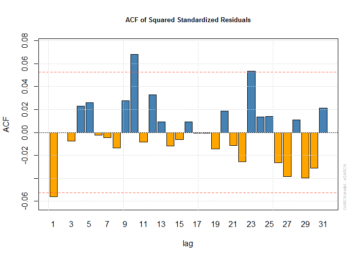
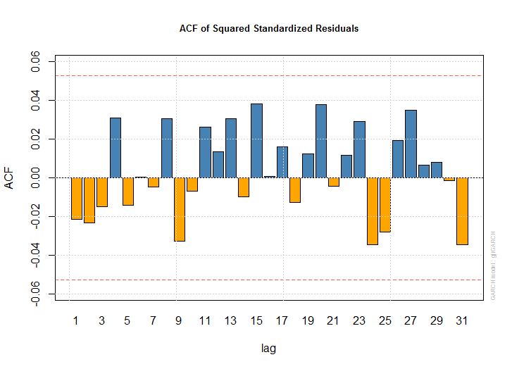
# GJR
dljp.spec<-ugarchspec(variance.model=list(model="gjrGARCH", garchOrder=c(1,1)), mean.model=list(armaOrder=c(1,0), include.mean=T))
dljp.gjr<-ugarchfit(data=dljp, spec=dljp.spec)
dljp.gjr
*---------------------------------*
*          GARCH Model Fit        *
*---------------------------------*

Conditional Variance Dynamics
-----------------------------------
GARCH Model	: gjrGARCH(1,1)
Mean Model	: ARFIMA(1,0,0)
Distribution	: norm

Optimal Parameters
------------------------------------
        Estimate  Std. Error   t value Pr(>|t|)
mu      0.000304    0.000304  0.999384 0.317609
ar1    -0.001567    0.028243 -0.055491 0.955747
omega   0.000007    0.000000 20.873872 0.000000
alpha1  0.017432    0.006800  2.563331 0.010367
beta1   0.877409    0.010546 83.198403 0.000000
gamma1  0.123741    0.025443  4.863400 0.000001

Robust Standard Errors:
        Estimate  Std. Error   t value Pr(>|t|)
mu      0.000304    0.000282   1.07554 0.282131
ar1    -0.001567    0.026541  -0.05905 0.952912
omega   0.000007    0.000000  24.15722 0.000000
alpha1  0.017432    0.007349   2.37207 0.017689
beta1   0.877409    0.008430 104.07677 0.000000
gamma1  0.123741    0.031752   3.89708 0.000097

LogLikelihood : 4162.846

Information Criteria
------------------------------------

Akaike       -5.9811
Bayes        -5.9585
Shibata      -5.9811
Hannan-Quinn -5.9726

Weighted Ljung-Box Test on Standardized Residuals
------------------------------------

*---------------------------------*
*          GARCH Model Fit        *
*---------------------------------*

Conditional Variance Dynamics
-----------------------------------
GARCH Model	: gjrGARCH(1,1)
Mean Model	: ARFIMA(1,0,0)
Distribution	: norm

Optimal Parameters
------------------------------------
        Estimate  Std. Error   t value Pr(>|t|)
mu      0.000304    0.000304  0.999384 0.317609
ar1    -0.001567    0.028243 -0.055491 0.955747
omega   0.000007    0.000000 20.873872 0.000000
alpha1  0.017432    0.006800  2.563331 0.010367
beta1   0.877409    0.010546 83.198403 0.000000
gamma1  0.123741    0.025443  4.863400 0.000001

Robust Standard Errors:
        Estimate  Std. Error   t value Pr(>|t|)
mu      0.000304    0.000282   1.07554 0.282131
ar1    -0.001567    0.026541  -0.05905 0.952912
omega   0.000007    0.000000  24.15722 0.000000
alpha1  0.017432    0.007349   2.37207 0.017689
beta1   0.877409    0.008430 104.07677 0.000000
gamma1  0.123741    0.031752   3.89708 0.000097

LogLikelihood : 4162.846

Information Criteria
------------------------------------

Akaike       -5.9811
Bayes        -5.9585
Shibata      -5.9811
Hannan-Quinn -5.9726

Weighted Ljung-Box Test on Standardized Residuals
------------------------------------
                        statistic p-value
Lag[1]                    0.07495  0.7843
Lag[2*(p+q)+(p+q)-1][2]   0.99937  0.7403
Lag[4*(p+q)+(p+q)-1][5]   1.76512  0.7776
d.o.f=1
H0 : No serial correlation

Weighted Ljung-Box Test on Standardized Squared Residuals
------------------------------------
                        statistic p-value
Lag[1]                     0.6437  0.4224
Lag[2*(p+q)+(p+q)-1][5]    2.0086  0.6164
Lag[4*(p+q)+(p+q)-1][9]    3.0480  0.7510
d.o.f=2

Weighted ARCH LM Tests
------------------------------------
            Statistic Shape Scale P-Value
ARCH Lag[3]    0.3121 0.500 2.000  0.5764
ARCH Lag[5]    1.5248 1.440 1.667  0.5858
ARCH Lag[7]    1.6458 2.315 1.543  0.7917

Nyblom stability test
------------------------------------
Joint Statistic:  21.5161
Individual Statistics:
mu     0.2835
ar1    0.8198
omega  4.1418
alpha1 0.2854
beta1  0.2736
gamma1 0.1365

Asymptotic Critical Values (10% 5% 1%)
Joint Statistic:     	 1.49 1.68 2.12
Individual Statistic:	 0.35 0.47 0.75

Sign Bias Test
------------------------------------
                        statistic p-value
Lag[1]                    0.07495  0.7843
Lag[2*(p+q)+(p+q)-1][2]   0.99937  0.7403
Lag[4*(p+q)+(p+q)-1][5]   1.76512  0.7776
d.o.f=1
H0 : No serial correlation

Weighted Ljung-Box Test on Standardized Squared Residuals
------------------------------------
                        statistic p-value
Lag[1]                     0.6437  0.4224
Lag[2*(p+q)+(p+q)-1][5]    2.0086  0.6164
Lag[4*(p+q)+(p+q)-1][9]    3.0480  0.7510
d.o.f=2

Weighted ARCH LM Tests
------------------------------------
            Statistic Shape Scale P-Value
ARCH Lag[3]    0.3121 0.500 2.000  0.5764
ARCH Lag[5]    1.5248 1.440 1.667  0.5858
ARCH Lag[7]    1.6458 2.315 1.543  0.7917

Nyblom stability test
------------------------------------
Joint Statistic:  21.5161
Individual Statistics:
mu     0.2835
ar1    0.8198
omega  4.1418
alpha1 0.2854
beta1  0.2736
gamma1 0.1365

Asymptotic Critical Values (10% 5% 1%)
Joint Statistic:     	 1.49 1.68 2.12
Individual Statistic:	 0.35 0.47 0.75

Sign Bias Test
------------------------------------
                   t-value   prob sig
Sign Bias           0.4724 0.6367
Negative Sign Bias  0.4875 0.6260
Positive Sign Bias  0.8604 0.3897
Joint Effect        2.1598 0.5399


Adjusted Pearson Goodness-of-Fit Test:
------------------------------------
  group statistic p-value(g-1)
1    20     25.08       0.1580
2    30     35.54       0.1874
3    40     36.42       0.5883
4    50     51.44       0.3785


Elapsed time : 0.350035
out<-data.frame()
omega<--0.361037
alpha<-0.017432
beta<-0.877409
gamma<-0.123741
ht<-seq(1,3)
for (ht1 in c(0.5,1,2)) {
  i<-1
  for (ut1 in -2:2) {
    ht[i]<-omega+beta*ht1+alpha*ut1^2+gamma*ut1^2*sign(ut1<0)
    i<-i+1
  }
  out<-rbind(out, ht)
}
names(out)<-c(-2, -1, 0, 1, 2)
row.names(out)<-c(0.5, 1, 2)
out
          -2        -1         0         1         2
0.5 1.003403 0.5798845 0.4387115 0.4561435 0.5084395
1   1.442108 1.0185890 0.8774160 0.8948480 0.9471440
2   2.319517 1.8959980 1.7548250 1.7722570 1.8245530
          -2        -1         0         1         2
0.5 1.003403 0.5798845 0.4387115 0.4561435 0.5084395
1   1.442108 1.0185890 0.8774160 0.8948480 0.9471440
2   2.319517 1.8959980 1.7548250 1.7722570 1.8245530
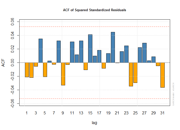
# EGARCH
dljp.spec<-ugarchspec(variance.model=list(model="eGARCH", garchOrder=c(1,1)), mean.model=list(armaOrder=c(1,0), include.mean=T))
dljp.egarch<-ugarchfit(data=dljp, spec=dljp.spec)
dljp.egarch
*---------------------------------*
*          GARCH Model Fit        *
*---------------------------------*

Conditional Variance Dynamics
-----------------------------------
GARCH Model	: eGARCH(1,1)
Mean Model	: ARFIMA(1,0,0)
Distribution	: norm

Optimal Parameters
------------------------------------
        Estimate  Std. Error  t value Pr(>|t|)
mu      0.000191    0.000377  0.50733 0.611924
ar1    -0.003791    0.029245 -0.12961 0.896873
omega  -0.361037    0.232596 -1.55220 0.120614
alpha1 -0.088885    0.037871 -2.34705 0.018923
beta1   0.958573    0.026242 36.52825 0.000000
gamma1  0.168848    0.079853  2.11450 0.034473

Robust Standard Errors:
        Estimate  Std. Error   t value Pr(>|t|)
mu      0.000191    0.000874  0.218611  0.82695
ar1    -0.003791    0.039681 -0.095524  0.92390
omega  -0.361037    0.898477 -0.401832  0.68781
alpha1 -0.088885    0.134327 -0.661703  0.50816
beta1   0.958573    0.101299  9.462813  0.00000
gamma1  0.168848    0.309855  0.544926  0.58581

LogLikelihood : 4162.689

Information Criteria
------------------------------------

Akaike       -5.9808
Bayes        -5.9582
Shibata      -5.9809
Hannan-Quinn -5.9724

Weighted Ljung-Box Test on Standardized Residuals
------------------------------------
                        statistic p-value
Lag[1]                     0.1264  0.7222
Lag[2*(p+q)+(p+q)-1][2]    1.2006  0.6159
Lag[4*(p+q)+(p+q)-1][5]    2.0282  0.7032
d.o.f=1
H0 : No serial correlation

Weighted Ljung-Box Test on Standardized Squared Residuals
------------------------------------
                        statistic p-value
Lag[1]                     0.6199  0.4311
Lag[2*(p+q)+(p+q)-1][5]    1.9735  0.6247
Lag[4*(p+q)+(p+q)-1][9]    3.1966  0.7261
d.o.f=2

Weighted ARCH LM Tests
------------------------------------
                        statistic p-value
Lag[1]                     0.1264  0.7222
Lag[2*(p+q)+(p+q)-1][2]    1.2006  0.6159
Lag[4*(p+q)+(p+q)-1][5]    2.0282  0.7032
d.o.f=1
H0 : No serial correlation

Weighted Ljung-Box Test on Standardized Squared Residuals
------------------------------------
                        statistic p-value
Lag[1]                     0.6199  0.4311
Lag[2*(p+q)+(p+q)-1][5]    1.9735  0.6247
Lag[4*(p+q)+(p+q)-1][9]    3.1966  0.7261
d.o.f=2

Weighted ARCH LM Tests
------------------------------------
            Statistic Shape Scale P-Value
ARCH Lag[3]   0.04281 0.500 2.000  0.8361
ARCH Lag[5]   1.73869 1.440 1.667  0.5319
ARCH Lag[7]   1.91168 2.315 1.543  0.7360

Nyblom stability test
------------------------------------
Joint Statistic:  1.6343
Individual Statistics:
mu     0.32484
ar1    0.81875
omega  0.26270
alpha1 0.19614
beta1  0.26888
gamma1 0.02107

Asymptotic Critical Values (10% 5% 1%)
Joint Statistic:     	 1.49 1.68 2.12
Individual Statistic:	 0.35 0.47 0.75

Sign Bias Test
------------------------------------
                   t-value   prob sig
Sign Bias           0.1859 0.8525
Negative Sign Bias  0.4346 0.6640
Positive Sign Bias  1.0319 0.3023
Joint Effect        1.9371 0.5856


Adjusted Pearson Goodness-of-Fit Test:
------------------------------------
  group statistic p-value(g-1)
1    20     33.02       0.0239
2    30     32.99       0.2780
3    40     41.02       0.3820
4    50     49.14       0.4676


Elapsed time : 0.663059
out<-data.frame()
omega<-0.000191
alpha<--0.088884
beta<-0.958573
gamma<-0.168848
ht<-seq(1,3)
for (ht1 in c(0.5,1,2)) {
  i<-1
  for (ut1 in -2:2) {
    ht[i]<-omega+beta*ht1+alpha*ut1^2+gamma*ut1^2*sign(ut1<0)
    i<-i+1
  }
  out<-rbind(out, ht)
}
names(out)<-c(-2, -1, 0, 1, 2)
row.names(out)<-c(0.5, 1, 2)
out
           -2        -1         0         1          2
0.5 0.4381015 0.1982125 0.1182495 0.0293645 -0.2372905
1   0.9173880 0.6774990 0.5975360 0.5086510  0.2419960
2   1.8759610 1.6360720 1.5561090 1.4672240  1.2005690
           -2        -1         0         1          2
0.5 0.4381015 0.1982125 0.1182495 0.0293645 -0.2372905
1   0.9173880 0.6774990 0.5975360 0.5086510  0.2419960
2   1.8759610 1.6360720 1.5561090 1.4672240  1.2005690
- 11を選択
plot(dljp.garch)
plot(dljp.gjr)
plot(dljp.egarch)
7.5
DVEC, BEKK, CCC
- 他のモデルの関数が分からずCCCモデルのみ
library(ccgarch)

msci_day<-read.table("msci_day.txt",header=T)
jp<-msci_day$jp
uk<-msci_day$uk
us<-msci_day$us
data<-as.matrix(msci_day[,6:8])
a<-c(0.003, 0.005, 0.001)
A<-diag(c(0.2, 0.3, 0.15))
B<-diag(c(0.79, 0.6, 0.8))
R<-matrix(c(cor(jp,jp), cor(jp,uk), cor(jp,us), cor(uk,jp), cor(uk,uk), cor(uk,us), cor(us,jp), cor(us,uk), cor(us,us)), 3, 3)
eccc.estimation(a, A, B, R, data, model="diagonal")
でよいと思うが、
Error in solve.default(H) :
  system is computationally singular: reciprocal condition number = 1.26294e-21
Error in solve.default(H) :
  system is computationally singular: reciprocal condition number = 1.26294e-21