画像認識に使われる畳み込みニューラルネットワーク(以下CNNと呼ぶ)というものがあります。Tensorflow のチュートリアル(Deep MNIST for Experts)にも出てきますが、ネットワークが複雑で理解するのに苦労します。そこで、畳み込み層とプーリング層の中身を画像化して、何が行われているのかなんとなく体感したいと思います。
ベースとなる Deep MNIST for Experts のコード
今回使用するコードは github(tf-cnn-image) に上げてあります。
まずはCNNのコードを用意します。Deep MNIST for Expertsのコードから不要な箇所を削除したものを用意しました。コメントは最小限にしてあるので、詳しい動作を知りたい場合はこちらなどを参考にしてください。
# -*- coding: utf-8 -*-
import sys
sys.path.append('tensorflow/tensorflow/examples/tutorials/mnist')
import input_data
import tensorflow as tf


def weight_variable(shape):
    initial = tf.truncated_normal(shape, stddev=0.1)
    return tf.Variable(initial)


def bias_variable(shape):
    initial = tf.constant(0.1, shape=shape)
    return tf.Variable(initial)


def conv2d(x, W):
    return tf.nn.conv2d(x, W, strides=[1, 1, 1, 1], padding='SAME')


def max_pool_2x2(x):
    return tf.nn.max_pool(x, ksize=[1, 2, 2, 1],
                          strides=[1, 2, 2, 1], padding='SAME')


mnist = input_data.read_data_sets("MNIST_data/", one_hot=True)
x = tf.placeholder("float", shape=[None, 784])
y_ = tf.placeholder("float", shape=[None, 10])

"""
第1層
"""
W_conv1 = weight_variable([5, 5, 1, 32])
b_conv1 = bias_variable([32])
x_image = tf.reshape(x, [-1, 28, 28, 1])
h_conv1 = tf.nn.relu(conv2d(x_image, W_conv1) + b_conv1)
h_pool1 = max_pool_2x2(h_conv1)

"""
第2層
"""
W_conv2 = weight_variable([5, 5, 32, 64])
b_conv2 = bias_variable([64])
h_conv2 = tf.nn.relu(conv2d(h_pool1, W_conv2) + b_conv2)
h_pool2 = max_pool_2x2(h_conv2)

"""
全結合層への変換
"""
W_fc1 = weight_variable([7 * 7 * 64, 1024])
b_fc1 = bias_variable([1024])
h_pool2_flat = tf.reshape(h_pool2, [-1, 7 * 7 * 64])
h_fc1 = tf.nn.relu(tf.matmul(h_pool2_flat, W_fc1) + b_fc1)

"""
Dropout
"""
keep_prob = tf.placeholder("float")
h_fc1_drop = tf.nn.dropout(h_fc1, keep_prob)

"""
読み出し層
"""
W_fc2 = weight_variable([1024, 10])
b_fc2 = bias_variable([10])
y_conv = tf.nn.softmax(tf.matmul(h_fc1_drop, W_fc2) + b_fc2)

"""
モデルの学習
"""
cross_entropy = -tf.reduce_sum(y_ * tf.log(y_conv))
train_step = tf.train.AdamOptimizer(1e-4).minimize(cross_entropy)

"""
モデルの評価
"""
correct_prediction = tf.equal(tf.argmax(y_conv, 1), tf.argmax(y_, 1))
accuracy = tf.reduce_mean(tf.cast(correct_prediction, "float"))

with tf.Session() as sess:
    sess.run(tf.global_variables_initializer())
    for i in range(20000):
        batch = mnist.train.next_batch(50)
        if i % 100 == 0:
            train_accuracy = accuracy.eval(feed_dict={
                x: batch[0], y_: batch[1], keep_prob: 1.0})
            print("step %d, training accuracy %g" % (i, train_accuracy))
        train_step.run(feed_dict={x: batch[0], y_: batch[1], keep_prob: 0.5})

    print("test accuracy %g" % accuracy.eval(feed_dict={
        x: mnist.test.images, y_: mnist.test.labels, keep_prob: 1.0}))
ネットワーク各層の出力形式を表示してみる
CNNには第一層の畳み込み層とプーリング層、そして第二層と結合層と続きます。各層がどのような形式になっているのか確認してみます。
with tf.Session() as sess:
    sess.run(tf.global_variables_initializer())
    batch = mnist.train.next_batch(50)
    feed_dict = {x: batch[0], y_: batch[1], keep_prob: 1.0}

    print("W_conv1: ", W_conv1.eval().shape)
    print("b_conv1: ", b_conv1.eval().shape)
    print("x_image: ", x_image.eval(feed_dict=feed_dict).shape)
    print("h_conv1: ", h_conv1.eval(feed_dict=feed_dict).shape)
    print("h_pool1: ", h_pool1.eval(feed_dict=feed_dict).shape)

    print("W_conv2: ", W_conv2.eval().shape)
    print("b_conv2: ", b_conv2.eval().shape)
    print("h_conv2: ", h_conv2.eval(feed_dict=feed_dict).shape)
    print("h_pool2: ", h_pool2.eval(feed_dict=feed_dict).shape)

    print("W_fc1: ", W_fc1.eval().shape)
    print("b_fc1: ", b_fc1.eval().shape)
    print("h_pool2_flat: ", h_pool2_flat.eval(feed_dict=feed_dict).shape)
    print("h_fc1: ", h_fc1.eval(feed_dict=feed_dict).shape)

    print("h_fc1_drop: ", h_fc1_drop.eval(feed_dict=feed_dict).shape)

    print("W_fc2: ", W_fc2.eval().shape)
    print("b_fc2: ", b_fc2.eval().shape)
    print("y_conv: ", y_conv.eval(feed_dict=feed_dict).shape)

# W_conv1:  (5, 5, 1, 32)
# b_conv1:  (32,)
# x_image:  (50, 28, 28, 1)
# h_conv1:  (50, 28, 28, 32)
# h_pool1:  (50, 14, 14, 32)
# W_conv2:  (5, 5, 32, 64)
# b_conv2:  (64,)
# h_conv2:  (50, 14, 14, 64)
# h_pool2:  (50, 7, 7, 64)
# W_fc1:  (3136, 1024)
# b_fc1:  (1024,)
# h_pool2_flat:  (50, 3136)
# h_fc1:  (50, 1024)
# h_fc1_drop:  (50, 1024)
# W_fc2:  (1024, 10)
# b_fc2:  (10,)
# y_conv:  (50, 10)
それぞれの層の計算結果は W_conv1.eval() のように eval() メソッドを呼び出すことで取得できます。print("W_conv1: ", W_conv1.eval().shape) とすると結果(行列)の型が取得できます。
print("W_conv1: ", W_conv1.eval().shape)
# W_conv1:  (5, 5, 1, 32)
これは 5 x 5 x 1 x 32 の配列(行列)が計算結果として返ってきたことになります。
shape を付けずにprintすれば中身の確認もできます。
print("W_conv1: ", W_conv1.eval())
"""
W_conv1:  [[[[ -1.23130225e-01  -1.35876462e-02   4.32779454e-03   7.67905191e-02
      9.60119516e-02  -1.52146637e-01  -1.95266187e-01  -3.94680016e-02
      7.22171217e-02  -8.30523148e-02   1.21835567e-01  -1.77600980e-01
      2.14710459e-02  -8.71937573e-02  -1.44006601e-02  -8.36562514e-02
     -1.46166608e-01  -4.43873368e-03   9.04049501e-02   1.72778830e-01
     -1.87566504e-01   1.45240754e-01   4.66598086e-02  -5.61284199e-02
     -9.03827175e-02   2.92096492e-02   4.94740643e-02  -2.18347758e-02
      1.74995847e-02  -6.22901395e-02   6.10287003e-02   1.21927358e-01]]
-- 省略 --
"""
画像化するのは畳み込み層とプーリング層なので以下の計算結果を使うことになります。
# h_conv1:  (50, 28, 28, 32)
# h_pool1:  (50, 14, 14, 32)
# h_conv2:  (50, 14, 14, 64)
# h_pool2:  (50, 7, 7, 64)
ちなみに、どれも先頭の次元が50ですが、これはミニバッチ処理として画像を50枚づつ与えて計算しているからです。そして h_conv1 では 28 x 28 のサイズの画像を作り、h_pool1 と h_conv2 では 14 x 14 の画像を作り、h_pool2 では 7 x 7 の画像を作ります。
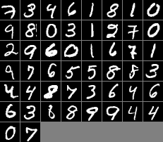
画像の作り方
Python3.5で実装しているので画像の作成ツールとしてPillowを使用します。Tensorflowの計算結果はnumpy.arrayですが、そこからPillowで画像を作るのはとても簡単なのですが多少修正してあげる必要があります。まずは入力データである元データを画像化してみようと思います。
with tf.Session() as sess:
    sess.run(tf.global_variables_initializer())
    batch = mnist.train.next_batch(50)
    images = x_image.eval(feed_dict={x: batch[0], y_: batch[1], keep_prob: 1.0})
    #print(images)
    #print(images.shape)
    images = images.reshape((-1, 28, 28)) * 255
    save_image("2.png", images)
def save_image(file_name, image_ndarray, cols=8):
    # 画像数, 幅, 高さ
    count, w, h = image_ndarray.shape
    # 縦に画像を配置する数
    rows = int((count - 1) / cols) + 1
    # 復数の画像を大きな画像に配置し直す
    canvas = Image.new("RGB", (w * cols + (cols - 1), h * rows + (rows - 1)), (0x80, 0x80, 0x80))
    for i, image in enumerate(image_ndarray):
        # 横の配置座標
        x_i = int(i % cols)
        x = int(x_i * w + x_i * 1)
        # 縦の配置座標
        y_i = int(i / cols)
        y = int(y_i * h + y_i * 1)
        out_image = Image.fromarray(np.uint8(image))
        canvas.paste(out_image, (x, y))
    canvas.save('images/' + file_name, "PNG")
まず元画像の層は x_image なので、そのデータを取得します。
images = x_image.eval(feed_dict={x: batch[0], y_: batch[1], keep_prob: 1.0})
このデータの型は (50, 28, 28, 1) になります。これを (50, 28, 28) に変え、かつデータは0〜1.0の値で入っているので、これを0〜255に変換します。
images = images.reshape((-1, 28, 28)) * 255
save_image() では、まず50枚全ての画像を敷き詰める空の画像を Image.new() で作成します。その後 Image.fromarray() でnumpy.arrayから個別の画像を作成し、 canvas.paste() で画像を敷き詰めていきます。このような画像が作成されます。
畳み込み層とプーリング層の画像を作成
それでは畳み込み層とプーリング層の画像を作成してきたいと思いますが、ディープラーニングでは学習を続けると各層のウェイト値とバイアス値が最適な値に調整されていき賢いAIが作られます。畳み込み層とプーリング層もウェイト値とバイアス値によって異なるものができるので、未学習な状態で作られる画像と、学習後の状態で作られる画像を作成し比較してみようと思います。
def train():
    for i in range(20000):
        batch = mnist.train.next_batch(50)
        if i % 100 == 0:
            train_accuracy = accuracy.eval(feed_dict={
                x: batch[0], y_: batch[1], keep_prob: 1.0})
            print("step %d, training accuracy %g" % (i, train_accuracy))
        train_step.run(feed_dict={x: batch[0], y_: batch[1], keep_prob: 0.5})

    print("test accuracy %g" % accuracy.eval(feed_dict={
        x: mnist.test.images, y_: mnist.test.labels, keep_prob: 1.0}))


def create_images(tag):
    batch = mnist.train.next_batch(10)
    feed_dict = {x: batch[0], keep_prob: 1.0}

    # 畳み込み1層
    h_conv1_result = h_conv1.eval(feed_dict=feed_dict)
    for i, result in enumerate(h_conv1_result):
        images = channels_to_images(result)
        save_image("3_%s_h_conv1_%02d.png" % (tag, i), images)

    # プーリング1層
    h_pool1_result = h_pool1.eval(feed_dict=feed_dict)
    for i, result in enumerate(h_pool1_result):
        images = channels_to_images(result)
        save_image("3_%s_h_pool1_%02d.png" % (tag, i), images)

    # 畳み込み2層
    h_conv2_result = h_conv2.eval(feed_dict=feed_dict)
    for i, result in enumerate(h_conv2_result):
        images = channels_to_images(result)
        save_image("3_%s_h_conv2_%02d.png" % (tag, i), images)

    # プーリング2層
    h_pool2_result = h_pool2.eval(feed_dict=feed_dict)
    for i, result in enumerate(h_pool2_result):
        images = channels_to_images(result)
        save_image("3_%s_h_pool2_%02d.png" % (tag, i), images)

    print("Created images. tag =", tag)
    print("Number: ", [v.argmax() for v in batch[1]])


with tf.Session() as sess:
    sess.run(tf.global_variables_initializer())
    # 画像作成
    create_images("before")
    # トレーニング
    train()
    # 画像作成
    create_images("after")
学習前と後で画像を作ります。
    # 画像作成
    create_images("before")
    # トレーニング
    train()
    # 画像作成
    create_images("after")
create_images() では各層の h_conv1 h_pool1 h_conv2 h_pool2 と、入力の画像毎に出力の画像を作成します。
def create_images(tag):
    batch = mnist.train.next_batch(10)
    feed_dict = {x: batch[0], keep_prob: 1.0}

    # 畳み込み1層
    h_conv1_result = h_conv1.eval(feed_dict=feed_dict)
    for i, result in enumerate(h_conv1_result):
        images = channels_to_images(result)
        save_image("3_%s_h_conv1_%02d.png" % (tag, i), images)
入力画像はあまり多くても意味がないので10枚 mnist.train.next_batch(10) にします。h_conv1_result には (10, 28, 28, 32) という形式で結果が返ります。これは10枚の入力画像に対して 28 x 28 のデータが32種類(チャンネル)という意味になります。この型では画像にできないので channels_to_images() で各入力画像ごとに (32, 28, 28) という型に変換します。
def channels_to_images(channels):
    count = channels.shape[2]
    images = []
    for i in range(count):
        image = []
        for line in channels:
            out_line = [pix[i] for pix in line]
            image.append(out_line)
        images.append(image)
    return np.array(images) * 255
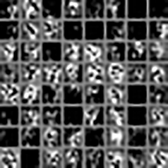
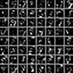
これで、このように28x28のサイズの画像32枚を敷き詰めた画像が10枚(入力画像数分)作成されます。
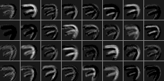
h_pool2 のプーリング第二層だと7x7のサイズの画像が64枚なので、こんな小さいものになります。

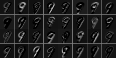
比較してみる
入力が9の画像だった場合の結果を比較してみます。見やすいようにオリジナル画像を拡大してあります。
第一畳み込み層
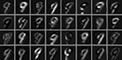
学習前
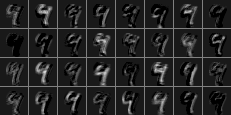
学習後
第一プーリング層
学習前
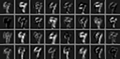
学習後
第二畳み込み層
学習前
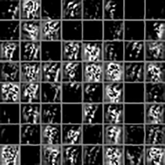
学習後
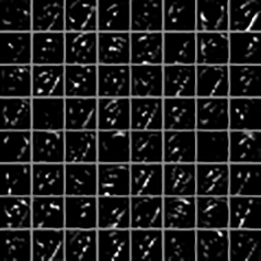
第二プーリング層
学習前
学習後
感想
なんとなく、、学習しているような気がする。。。たぶん。。。なんか大きくノイズっぽい塊だったのが、それとなくどこかの特徴を見出しているような、、、よくわからないけど。。。それがディープラーニングなんだろうきっと
簡単実行
tf-cnn-image を落としたら以下のように実行できます。
$ python 0.py
$ python 1.py
$ python 2.py
$ python 3.py