この記事の続きです。
本記事で使用したコードはこちら。
準備
前編と同じなので、コードは折りたたんでおきます。なお、今回動かしていたPolarsのバージョンは0.15.13です。
展開
!pip install polars
import os
import polars as pl
import math
from sklearn import preprocessing
from sklearn import model_selection

if not os.path.exists('../data/'):
    !git clone https://github.com/The-Japan-DataScientist-Society/100knocks-preprocess
    os.chdir('100knocks-preprocess/docker/work/answer')

dtypes = {
    'customer_id': str,
    'gender_cd': str,
    'postal_cd': str,
    'application_store_cd': str,
    'status_cd': str,
    'category_major_cd': str,
    'category_medium_cd': str,
    'category_small_cd': str,
    'product_cd': str,
    'store_cd': str,
    'prefecture_cd': str,
    'tel_no': str,
    'postal_cd': str,
    'street': str,
    'application_date': str,
    'birth_day': pl.Date
}

df_customer = pl.read_csv("../data/customer.csv", dtypes=dtypes)
df_category = pl.read_csv("../data/category.csv", dtypes=dtypes)
df_product = pl.read_csv("../data/product.csv", dtypes=dtypes)
df_receipt = pl.read_csv("../data/receipt.csv", dtypes=dtypes)
df_store = pl.read_csv("../data/store.csv", dtypes=dtypes)
df_geocode = pl.read_csv("../data/geocode.csv", dtypes=dtypes)
なお、一部 scikit-learn を使用して書いている問題があります。
P-051 ~ P-060
P-051:
レシート明細データ(df_receipt)の売上エポック秒を日付型に変換し、「日」だけ取り出してレシート番号(receipt_no)、レシートサブ番号(receipt_sub_no)とともに10件表示せよ。なお、「日」は0埋め2桁で取り出すこと。
df_receipt.select([
    'receipt_no',
    'receipt_sub_no',
    (pl.col('sales_epoch').cast(pl.Utf8)
        .str.strptime(pl.Datetime, fmt='%s').dt.strftime('%d')
    ).alias('sales_day')
]).head(10)
P-052:
レシート明細データ(df_receipt)の売上金額(amount)を顧客ID(customer_id)ごとに合計の上、売上金額合計に対して2,000円以下を0、2,000円より大きい金額を1に二値化し、顧客ID、売上金額合計とともに10件表示せよ。ただし、顧客IDが"Z"から始まるのものは非会員を表すため、除外して計算すること。
df_receipt.filter(
    pl.col('customer_id').str.starts_with('Z').is_not()
).groupby('customer_id').agg(
    pl.col('amount').sum()
).select([
    'customer_id',
    'amount',
    pl.when(pl.col('amount') > 2000).then(1).otherwise(0).alias('sales_flg')
]).sort('customer_id').head(10)
こちらの when ~ then ~ otherwise が、Pandasと大きく異なる機能のひとつです。when ~ then を複数回つなげて書くこともできます。
P-053:
顧客データ(df_customer)の郵便番号(postal_cd)に対し、東京(先頭3桁が100〜209のもの)を1、それ以外のものを0に二値化せよ。さらにレシート明細データ(df_receipt)と結合し、全期間において売上実績のある顧客数を、作成した二値ごとにカウントせよ。
df_customer.with_column(
    pl.when(pl.col('postal_cd').str.slice(0, 3).
            cast(pl.Int16).is_between(100, 209, closed='both'))
    .then(1)
    .otherwise(0).alias('is_tokyo')
).join(
    df_receipt, on='customer_id', how='inner'
).groupby('is_tokyo').agg(
    pl.col('customer_id').n_unique()
)
P-054:
顧客データ(df_customer)の住所(address)は、埼玉県、千葉県、東京都、神奈川県のいずれかとなっている。都道府県毎にコード値を作成し、顧客ID、住所とともに10件表示せよ。値は埼玉県を11、千葉県を12、東京都を13、神奈川県を14とすること。
df_customer.with_column(
    pl.when(pl.col('address').str.contains('埼玉県'))
    .then(11)
    .when(pl.col('address').str.contains('千葉県'))
    .then(12)
    .when(pl.col('address').str.contains('東京都'))
    .then(13)
    .when(pl.col('address').str.contains('神奈川県'))
    .then(14).alias('prefecture')
).select([
    'customer_id',
    'address',
    'prefecture'
]).head(10)
ここでは特に理由もなく with_column で列作成していますが、select の中で書いてももちろん大丈夫です。
以下に str.replace を用いた別解を書いておきます。前編 のP-043も参考になるかと思います。
df_customer.with_column(
    pl.col('address').str.replace(r'埼玉県.*', '11')
    .str.replace(r'千葉県.*', '12')
    .str.replace(r'東京都.*', '13')
    .str.replace(r'神奈川県.*', '14')
    .cast(pl.Int16).alias('prefecture')
).select([
    'customer_id',
    'address',
    'prefecture'
]).head(10)
P-055:
レシート明細(df_receipt)データの売上金額(amount)を顧客ID(customer_id)ごとに合計し、その合計金額の四分位点を求めよ。その上で、顧客ごとの売上金額合計に対して以下の基準でカテゴリ値を作成し、顧客ID、売上金額合計とともに10件表示せよ。カテゴリ値は順に1〜4とする。
- 最小値以上第1四分位未満 ・・・ 1を付与
- 第1四分位以上第2四分位未満 ・・・ 2を付与
- 第2四分位以上第3四分位未満 ・・・ 3を付与
- 第3四分位以上 ・・・ 4を付与
df_receipt.groupby('customer_id').agg(
    pl.col('amount').sum()
).with_column(
    pl.when(pl.col('amount') < pl.col('amount').quantile(0.25))
    .then(1)
    .when(pl.col('amount') < pl.col('amount').quantile(0.5))
    .then(2)
    .when(pl.col('amount') < pl.col('amount').quantile(0.75))
    .then(3)
    .otherwise(4).alias('pct_group')
).sort('customer_id').head(10)
もっと条件分岐の数が多くて when ~ then を繰り返すのが面倒な時は、こんな感じで(クソ雑コードですが…)pl.Exprを返す関数を作るのもありでしょう。
def cut_quantile(col: str, bins: list) -> pl.Expr:
    expr = pl
    for n, bin in enumerate(bins):
        expr = expr.when(pl.col(col) < pl.col(col).quantile(bin)).then(n + 1)
    expr = expr.otherwise(n + 2)
    return expr

df_receipt.groupby('customer_id').agg(
    pl.col('amount').sum()
).with_column(
    cut_quantile('amount', [0.25, 0.5, 0.75]).alias('pct_group')
).sort('customer_id').head(10)
P-056:
顧客データ(df_customer)の年齢(age)をもとに10歳刻みで年代を算出し、顧客ID(customer_id)、生年月日(birth_day)とともに10件表示せよ。ただし、60歳以上は全て60歳代とすること。年代を表すカテゴリ名は任意とする。
df_customer.select([
    'customer_id',
    'birth_day',
    (pl.when(pl.col('age') >= 60)
    .then(60)
    .otherwise(pl.col('age')) / 10).floor().alias('era')
]).head(10)
もちろん以下のように apply を使う方法もあります。
df_customer.select([
    'customer_id',
    'birth_day',
    pl.col('age').apply(lambda x: math.floor(min(x, 60) / 10)).alias('era')
]).head(10)
P-057:
056の抽出結果と性別コード(gender_cd)により、新たに性別×年代の組み合わせを表すカテゴリデータを作成し、10件表示せよ。組み合わせを表すカテゴリの値は任意とする。
df_customer.with_column(
    (pl.when(pl.col('age') >= 60)
    .then(60)
    .otherwise(pl.col('age')) / 10).cast(pl.Int8).alias('era')
).select([
    'customer_id',
    'birth_day',
    'age',
    'gender_cd',
    pl.concat_str([
        pl.col('era'), pl.col('gender_cd')
    ], sep='_').alias('demographics')
]).head(10)
文字列として結合しています。
Int型にcastしてることに特に意味はないです(小数点以下まで残るのが見栄えが悪くて嫌だっただけ)。
P-058:
顧客データ(df_customer)の性別コード(gender_cd)をダミー変数化し、顧客ID(customer_id)とともに10件表示せよ。
df_customer.select([
    'customer_id',
    *pl.get_dummies(df_customer.select('gender_cd'))
]).head(10)
3行目の頭で*をつけてる理由を説明します。
pl.get_dummies(df_customer.select('gender_cd'))は、pl.DataFrameを生成します。
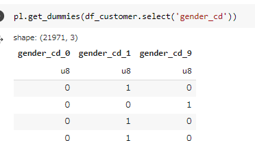
一方、select が受け付けるのはpl.Exprやpl.Seriesなどで、pl.DataFrameは受け付けません。そこで、pl.DataFrameをpl.Seriesが格納されたリストにすることで select に渡せるようにしたいです。pl.DataFrameはiterableなので、*を付けることでアンパックしてSeriesのリストにしています1。
P-059:
レシート明細データ(df_receipt)の売上金額(amount)を顧客ID(customer_id)ごとに合計し、売上金額合計を平均0、標準偏差1に標準化して顧客ID、売上金額合計とともに10件表示せよ。標準化に使用する標準偏差は、分散の平方根、もしくは不偏分散の平方根のどちらでも良いものとする。ただし、顧客IDが"Z"から始まるのものは非会員を表すため、除外して計算すること。
amount = pl.col('amount')

df_receipt.filter(
    pl.col('customer_id').str.starts_with('Z').is_not()
).groupby('customer_id').agg(
    pl.col('amount').sum()
).select([
    'customer_id',
    'amount',
    ((amount - amount.mean()) / amount.std(ddof=0)).alias('std_amount')
]).sort('customer_id').head(10)
pl.col('amount') の登場回数がやけに多いので取り出しています。
sklearnを使う別解は以下の通りです。
df_sales_amount = df_receipt.filter(
    pl.col('customer_id').str.starts_with('Z').is_not()
).groupby('customer_id').agg(
    pl.col('amount').sum()
).sort('customer_id')

df_sales_amount.with_columns(
    *pl.from_numpy(
        preprocessing.StandardScaler().fit_transform(
            df_sales_amount.select('amount').to_numpy()
        ),
        columns=['std_amount']
    )
).head(10)
StandardScaler().fit() にpolarsのDataFrameを渡すことはできなかったので、numpyオブジェクトに変換してから渡しています。*を付けている理由は、ひとつ前のP-058と同じです。
P-060:
レシート明細データ(df_receipt)の売上金額(amount)を顧客ID(customer_id)ごとに合計し、売上金額合計を最小値0、最大値1に正規化して顧客ID、売上金額合計とともに10件表示せよ。ただし、顧客IDが"Z"から始まるのものは非会員を表すため、除外して計算すること。
def minmax_scale(c: str) -> pl.Expr:
    return (pl.col(c) - pl.col(c).min()) / (pl.col(c).max() - pl.col(c).min())

df_receipt.filter(
    pl.col('customer_id').str.starts_with('Z').is_not()
).groupby('customer_id').agg(
    pl.col('amount').sum()
).select([
    'customer_id',
    'amount',
    minmax_scale('amount').alias('amount_scale')
]).sort('customer_id').head(10)
P-061 ~ P-070
P-061:
レシート明細データ(df_receipt)の売上金額(amount)を顧客ID(customer_id)ごとに合計し、売上金額合計を常用対数化(底10)して顧客ID、売上金額合計とともに10件表示せよ。ただし、顧客IDが"Z"から始まるのものは非会員を表すため、除外して計算すること。
df_receipt.filter(
    pl.col('customer_id').str.starts_with('Z').is_not()
).groupby('customer_id').agg(
    pl.col('amount').sum()
).select([
    'customer_id',
    'amount',
    pl.col('amount').log10().alias('log10_amount')
]).sort('customer_id').head(10)
P-062:
レシート明細データ(df_receipt)の売上金額(amount)を顧客ID(customer_id)ごとに合計し、売上金額合計を自然対数化(底e)して顧客ID、売上金額合計とともに10件表示せよ。ただし、顧客IDが"Z"から始まるのものは非会員を表すため、除外して計算すること。
df_receipt.filter(
    pl.col('customer_id').str.starts_with('Z').is_not()
).groupby('customer_id').agg(
    pl.col('amount').sum()
).select([
    'customer_id',
    'amount',
    pl.col('amount').log().alias('log_amount')
]).sort('customer_id').head(10)
P-063:
商品データ(df_product)の単価(unit_price)と原価(unit_cost)から各商品の利益額を算出し、結果を10件表示せよ。
df_product.with_column(
    (pl.col('unit_price') - pl.col('unit_cost')).alias('unit_profit')
).head(10)
P-064:
商品データ(df_product)の単価(unit_price)と原価(unit_cost)から、各商品の利益率の全体平均を算出せよ。ただし、単価と原価には欠損が生じていることに注意せよ。
df_product.select(
    ((pl.col('unit_price') - pl.col('unit_cost')) / pl.col('unit_price'))
    .alias('unit_profit_rate').mean()
)
polarsだと groupby を挟まないテーブル全体での集計には select を使います。以下のように pl.DataFrame に対するメソッドを使っても同じ結果となります。
df_product.select(
    ((pl.col('unit_price') - pl.col('unit_cost')) / pl.col('unit_price'))
    .alias('unit_profit_rate')
).mean()
P-065:
商品データ(df_product)の各商品について、利益率が30%となる新たな単価を求めよ。ただし、1円未満は切り捨てること。そして結果を10件表示させ、利益率がおよそ30%付近であることを確認せよ。ただし、単価(unit_price)と原価(unit_cost)には欠損が生じていることに注意せよ。
df_product.with_column(
    ((pl.col('unit_cost') / 0.7).floor()).alias('new_price')
).with_column(
    ((pl.col('new_price') - pl.col('unit_cost')) / pl.col('new_price')).alias('new_profit_rate')
).head(10)
with_columns は自身の中で作成したカラムにアクセスできないので、このケースでは with_column を2回に分けて書く必要があります。
P-066:
商品データ(df_product)の各商品について、利益率が30%となる新たな単価を求めよ。今回は、1円未満を丸めること(四捨五入または偶数への丸めで良い)。そして結果を10件表示させ、利益率がおよそ30%付近であることを確認せよ。ただし、単価(unit_price)と原価(unit_cost)には欠損が生じていることに注意せよ。
df_product.with_column(
    ((pl.col('unit_cost') / 0.7).round(0)).alias('new_price')
).with_column(
    ((pl.col('new_price') - pl.col('unit_cost')) / pl.col('new_price')).alias('new_profit_rate')
).head(10)
P-067:
商品データ(df_product)の各商品について、利益率が30%となる新たな単価を求めよ。今回は、1円未満を切り上げること。そして結果を10件表示させ、利益率がおよそ30%付近であることを確認せよ。ただし、単価(unit_price)と原価(unit_cost)には欠損が生じていることに注意せよ。
df_product.with_column(
    ((pl.col('unit_cost') / 0.7).ceil()).alias('new_price')
).with_column(
    ((pl.col('new_price') - pl.col('unit_cost')) / pl.col('new_price')).alias('new_profit_rate')
).head(10)
P-068:
商品データ(df_product)の各商品について、消費税率10%の税込み金額を求めよ。1円未満の端数は切り捨てとし、結果を10件表示せよ。ただし、単価(unit_price)には欠損が生じていることに注意せよ。
df_product.select([
    'product_cd',
    'unit_price',
    ((pl.col('unit_price') * 1.1).floor()).alias('tax_price')
]).head(10)
P-069:
レシート明細データ(df_receipt)と商品データ(df_product)を結合し、顧客毎に全商品の売上金額合計と、カテゴリ大区分コード(category_major_cd)が"07"(瓶詰缶詰)の売上金額合計を計算の上、両者の比率を求めよ。抽出対象はカテゴリ大区分コード"07"(瓶詰缶詰)の売上実績がある顧客のみとし、結果を10件表示せよ。
df_receipt.join(
    df_product, how='inner', on='product_cd'
).groupby('customer_id').agg([
    (pl.col('quantity') * pl.col('unit_price')).sum().alias('amount_all'),
    (pl.col('quantity') * pl.col('unit_price')).filter(
        pl.col('category_major_cd')=='07'
    ).sum().alias('amount_07')
]).filter(
    pl.col('amount_07').is_not_null()
).with_column(
    (pl.col('amount_07') / pl.col('amount_all')).alias('sales_rate')
).sort('customer_id').head(10)
この例のように、pl.Exprの中で filter を使えるのはカラム作成の柔軟性という観点から便利です。
P-070:
レシート明細データ(df_receipt)の売上日(sales_ymd)に対し、顧客データ(df_customer)の会員申込日(application_date)からの経過日数を計算し、顧客ID(customer_id)、売上日、会員申込日とともに10件表示せよ(sales_ymdは数値、application_dateは文字列でデータを保持している点に注意)。
df_receipt.select([
    'customer_id',
    'sales_ymd'
]).unique().join(
    df_customer, on='customer_id', how='left'
).select([
    'customer_id',
    'sales_ymd',
    'application_date',
    (pl.col('sales_ymd').cast(str).str.strptime(pl.Date, '%Y%m%d') -
     pl.col('application_date').str.strptime(pl.Date, '%Y%m%d')).alias('elapsed_days')
]).head(10)
ここで計算しているような Date/Datetime 型の引き算の結果は、duration型になります。
P-071 ~ P-080
P-071:
レシート明細データ(df_receipt)の売上日(sales_ymd)に対し、顧客データ(df_customer)の会員申込日(application_date)からの経過月数を計算し、顧客ID(customer_id)、売上日、会員申込日とともに10件表示せよ(sales_ymdは数値、application_dateは文字列でデータを保持している点に注意)。1ヶ月未満は切り捨てること。
df_receipt.select([
    'customer_id',
    'sales_ymd'
]).unique().join(
    df_customer, on='customer_id', how='left'
).with_columns([
    pl.col('sales_ymd').cast(str).str.strptime(pl.Datetime, '%Y%m%d').alias('date1'),
    pl.col('application_date').str.strptime(pl.Datetime, '%Y%m%d').alias('date2')
]).select([
    'customer_id',
    'sales_ymd',
    'application_date',
    'date1',
    'date2',
    (
        (pl.col('date1').dt.year() - pl.col('date2').dt.year()) * 12 +
         pl.col('date1').dt.month() - pl.col('date2').dt.month()
    ).alias('elapsed_months'),
]).head(10)
月数の計算はそもそもどう定義するかもいくつか考えられ、なかなか難しい問題です…2
P-072:
レシート明細データ(df_receipt)の売上日(df_customer)に対し、顧客データ(df_customer)の会員申込日(application_date)からの経過年数を計算し、顧客ID(customer_id)、売上日、会員申込日とともに10件表示せよ(sales_ymdは数値、application_dateは文字列でデータを保持している点に注意)。1年未満は切り捨てること。
df_receipt.select([
    'customer_id',
    'sales_ymd'
]).unique().join(
    df_customer, on='customer_id', how='left'
).select([
    'customer_id',
    'sales_ymd',
    'application_date',
    ((pl.col('sales_ymd').cast(str).str.strptime(pl.Date, '%Y%m%d') -
      pl.col('application_date').str.strptime(pl.Date, '%Y%m%d')).dt.days() // 365).
    alias('elapsed_years')
]).head(10)
P-073:
レシート明細データ(df_receipt)の売上日(sales_ymd)に対し、顧客データ(df_customer)の会員申込日(application_date)からのエポック秒による経過時間を計算し、顧客ID(customer_id)、売上日、会員申込日とともに10件表示せよ(なお、sales_ymdは数値、application_dateは文字列でデータを保持している点に注意)。なお、時間情報は保有していないため各日付は0時0分0秒を表すものとする。
df_receipt.select([
    'customer_id',
    'sales_ymd'
]).unique().join(
    df_customer, on='customer_id', how='left'
).select([
    'customer_id',
    'sales_ymd',
    'application_date',
    (pl.col('sales_ymd').cast(str).str.strptime(pl.Datetime, '%Y%m%d').dt.epoch(tu='s') -
     pl.col('application_date').str.strptime(pl.Datetime, '%Y%m%d').dt.epoch(tu='s')).
    alias('elapsed_epoch')
]).head(10)
epoch秒単位で求めたい場合、以下のように差分をとってduration型にしてからepoch秒に直そうとするとうまく変換できない模様です。
(pl.col('sales_ymd').cast(str).str.strptime(pl.Datetime, '%Y%m%d') -
 pl.col('application_date').str.strptime(pl.Datetime, '%Y%m%d')
).dt.epoch(tu='s').alias('elapsed_epoch')
P-074:
レシート明細データ(df_receipt)の売上日(sales_ymd)に対し、当該週の月曜日からの経過日数を計算し、売上日、直前の月曜日付とともに10件表示せよ(sales_ymdは数値でデータを保持している点に注意)。
df_receipt.select([
    pl.col('sales_ymd').cast(str).str.strptime(pl.Date, '%Y%m%d'),
]).with_columns([
    pl.col('sales_ymd').dt.truncate('1w').alias('monday'),
    (pl.col('sales_ymd').dt.weekday() - 1).alias('elapsed_days')
]).head(10)
polarsの weekday は「月曜=1 ~ 日曜=7」となり、pandasと数字が1ずれるのは要注意です3
P-075:
顧客データ(df_customer)からランダムに1%のデータを抽出し、先頭から10件表示せよ。
df_customer.sample(frac=0.01).head(3)
P-076:
顧客データ(df_customer)から性別コード(gender_cd)の割合に基づきランダムに10%のデータを層化抽出し、性別コードごとに件数を集計せよ。
df_customer.groupby('gender_cd').apply(
    lambda x: x.sample(frac=0.1)
).select(
    pl.col('gender_cd').value_counts()
)
ここの groupby().apply() でやっていることは、apply の中の x にグループごとのpl.DataFrameが渡されて処理が走り、結果が再び結合されるイメージです。
P-077:
レシート明細データ(df_receipt)の売上金額を顧客単位に合計し、合計した売上金額の外れ値を抽出せよ。なお、外れ値は売上金額合計を対数化したうえで平均と標準偏差を計算し、その平均から3σを超えて離れたものとする(自然対数と常用対数のどちらでも可)。結果は10件表示せよ。
df_receipt.groupby('customer_id').agg(
    pl.col('amount').sum()
).with_column(
    pl.col('amount').log().alias('log_amount')
).filter(
    (pl.col('log_amount') - pl.col('log_amount').mean()).abs() >
    pl.col('log_amount').std() * 3
).head(10)
P-078:
レシート明細データ(df_receipt)の売上金額(amount)を顧客単位に合計し、合計した売上金額の外れ値を抽出せよ。ただし、顧客IDが"Z"から始まるのものは非会員を表すため、除外して計算すること。なお、ここでは外れ値を第1四分位と第3四分位の差であるIQRを用いて、「第1四分位数-1.5×IQR」を下回るもの、または「第3四分位数+1.5×IQR」を超えるものとする。結果は10件表示せよ。
df_receipt.filter(
    pl.col('customer_id').str.starts_with('Z').is_not()
).groupby('customer_id').agg(
    pl.col('amount').sum()
).with_columns([
    pl.col('amount').quantile(0.25).alias('1qtr'),
    pl.col('amount').quantile(0.75).alias('3qtr'),
    (pl.col('amount').quantile(0.75) - pl.col('amount').quantile(0.25)).alias('iqr'),
]).filter(
    (pl.col('amount') < pl.col('1qtr') - 1.5 * pl.col('iqr')) |
    (pl.col('amount') > pl.col('3qtr') + 1.5 * pl.col('iqr'))
).sort('customer_id').head(10)
長ったらしくなるので計算途中をカラムとして作っています。残るのが嫌なら最後に drop するのもありだし、次のような書き方もできます。
qtr1 = pl.col('amount').quantile(0.25)
qtr3 = pl.col('amount').quantile(0.75)

df_receipt.filter(
    pl.col('customer_id').str.starts_with('Z').is_not()
).groupby('customer_id').agg(
    pl.col('amount').sum()
).filter(
    (pl.col('amount') < qtr1 - 1.5 * (qtr3 - qtr1)) |
    (pl.col('amount') > qtr3 + 1.5 * (qtr3 - qtr1))
).sort('customer_id').head(10)
P-079:
商品データ(df_product)の各項目に対し、欠損数を確認せよ。
df_product.null_count()
P-080:
商品データ(df_product)のいずれかの項目に欠損が発生しているレコードを全て削除した新たな商品データを作成せよ。なお、削除前後の件数を表示させ、079で確認した件数だけ減少していることも確認すること。
df_product.drop_nulls()
# 結果確認
print(df_product.shape)
print(df_product.drop_nulls().shape)
P-081 ~ P-090
P-081:
単価(unit_price)と原価(unit_cost)の欠損値について、それぞれの平均値で補完した新たな商品データを作成せよ。なお、平均値については1円未満を丸めること(四捨五入または偶数への丸めで良い)。補完実施後、各項目について欠損が生じていないことも確認すること。
df_tmp = df_product.fill_null(strategy='mean')
df_tmp.null_count()
以下の書き方だと上手くいきません。value の引数に文字列で 'mean' を指定していると解釈されてしまいます。
df_tmp = df_product.fill_null('mean')
df_tmp.null_count()
P-082:
単価(unit_price)と原価(unit_cost)の欠損値について、それぞれの中央値で補完した新たな商品データを作成せよ。なお、中央値については1円未満を丸めること(四捨五入または偶数への丸めで良い)。補完実施後、各項目について欠損が生じていないことも確認すること。
df_tmp = df_product.select([
    pl.all().exclude(['unit_cost', 'unit_price']),
    pl.col('unit_cost').fill_null(pl.col('unit_cost').median().cast(pl.Int64)),
    pl.col('unit_price').fill_null(pl.median('unit_price').cast(pl.Int64)),
])

df_tmp.null_count()
pl.col('a').median() と pl.median('a') はどちらも同じことです。
median を噛ませると(偶数のときの処理の問題から)少数になりうるので、最後 cast でInt型に変換しています。
P-083:
単価(unit_price)と原価(unit_cost)の欠損値について、各商品のカテゴリ小区分コード(category_small_cd)ごとに算出した中央値で補完した新たな商品データを作成せよ。なお、中央値については1円未満を丸めること(四捨五入または偶数への丸めで良い)。補完実施後、各項目について欠損が生じていないことも確認すること。
df_tmp = df_product.select([
    pl.all().exclude(['unit_cost', 'unit_price']),
    pl.coalesce([
        pl.col('unit_cost'),
        pl.median('unit_cost').over('category_small_cd').cast(pl.Int64)
    ]),
    pl.coalesce([
        pl.col('unit_price'),
        pl.median('unit_price').over('category_small_cd').cast(pl.Int64)
    ]),
])
df_tmp.null_count()
over はPandasの groupby.transform に相当するものです。これはSQLライクな書き方に近く、Pandasとかなり異なる点です。
P-084:
顧客データ(df_customer)の全顧客に対して全期間の売上金額に占める2019年売上金額の割合を計算し、新たなデータを作成せよ。ただし、売上実績がない場合は0として扱うこと。そして計算した割合が0超のものを抽出し、結果を10件表示せよ。また、作成したデータに欠損が存在しないことを確認せよ。
df_tmp = df_customer.join(
    df_receipt.groupby('customer_id').agg([
        pl.col('amount').filter(
            pl.col('sales_ymd').is_between(20190000, 20191231, closed='both')
        ).sum().alias('amount_19'),
        pl.col('amount').sum().alias('amount_all'),
    ]).with_column(
        (pl.col('amount_19') / pl.col('amount_all')).alias('amount_rate')
    ),
    on='customer_id',
    how='left'
).fill_null(0)

df_tmp.filter(
    pl.col('amount_rate') > 0
).head(10)
# 欠損がないことを確認
df_tmp.null_count()
polarsのjoinに右外部結合(how=right)は存在しません。
P-085:
顧客データ(df_customer)の全顧客に対し、郵便番号(postal_cd)を用いてジオコードデータ(df_geocode)を紐付け、新たな顧客データを作成せよ。ただし、1つの郵便番号(postal_cd)に複数の経度(longitude)、緯度(latitude)情報が紐づく場合は、経度(longitude)、緯度(latitude)の平均値を算出して使用すること。また、作成結果を確認するために結果を10件表示せよ。
df_085 = df_customer.join(
    df_geocode.groupby('postal_cd').agg([
        pl.col('longitude').mean(),
        pl.col('latitude').mean(),
    ]),
    on='postal_cd', how='left'
)

df_085.head(10)
ここで作成したものを次の問題で使用するので、変数名をそれと分かるように書いています。
P-086:
085で作成した緯度経度つき顧客データに対し、会員申込店舗コード(application_store_cd)をキーに店舗データ(df_store)と結合せよ。そして申込み店舗の緯度(latitude)・経度情報(longitude)と顧客住所(address)の緯度・経度を用いて申込み店舗と顧客住所の距離(単位:km)を求め、顧客ID(customer_id)、顧客住所(address)、店舗住所(address)とともに表示せよ。計算式は以下の簡易式で良いものとするが、その他精度の高い方式を利用したライブラリを利用してもかまわない。結果は10件表示せよ。
\begin{aligned}
& \mbox{緯度(ラジアン)}:\phi \\
& \mbox{経度(ラジアン)}:\lambda \\
& \mbox{距離}L = 6371 * \arccos(\sin \phi_1 * \sin \phi_2 + \\
&  \cos \phi_1 * \cos \phi_2 * \cos(\lambda_1 − \lambda_2))
\end{aligned}
def distance_expr(lon1: str, lat1: str, lon2: str, lat2: str) -> pl.Expr:
    # radian = degrees * pi / 180
    lon1_rad = pl.col(lon1) * math.pi / 180
    lon2_rad = pl.col(lon2) * math.pi / 180
    lat1_rad = pl.col(lat1) * math.pi / 180
    lat2_rad = pl.col(lat2) * math.pi / 180

    return 6371 * (
        lat1_rad.sin() * lat2_rad.sin() +
        lat1_rad.cos() * lat2_rad.cos() * (lon1_rad - lon2_rad).cos()
    ).arccos()


df_085.join(
    df_store, how='inner', suffix='_store',
    left_on='application_store_cd', right_on='store_cd'
).select([
    'customer_id',
    'address',
    'address_store',
    distance_expr('longitude', 'latitude', 'longitude_store', 'latitude_store').alias('distance')
]).head(5)
suffixは右側のテーブル(joinメソッドの引数として渡したほう)に付きます。
P-087:
顧客データ(df_customer)では、異なる店舗での申込みなどにより同一顧客が複数登録されている。名前(customer_name)と郵便番号(postal_cd)が同じ顧客は同一顧客とみなして1顧客1レコードとなるように名寄せした名寄顧客データを作成し、顧客データの件数、名寄顧客データの件数、重複数を算出せよ。ただし、同一顧客に対しては売上金額合計が最も高いものを残し、売上金額合計が同一もしくは売上実績がない顧客については顧客ID(customer_id)の番号が小さいものを残すこととする。
df_087 = df_customer.join(
    df_receipt.groupby('customer_id').agg(
        pl.col('amount').sum()
    ),
    on='customer_id', how='left'
).sort(
    ['amount', 'customer_id'], reverse=[True, False]
).unique(subset=['customer_name', 'postal_cd'])

print('df_customer_cnt:', len(df_customer),
      '/ df_customer_unique_cnt:', len(df_087),
      '/ diff:', len(df_customer) - len(df_087))
sort で売上金額が多い順→顧客IDが小さいに並べ、unique はデフォルトだと最初の行を残すので、売上金額が最も高い(タイなら顧客IDが若い)ものが残ることになります。
P-088:
087で作成したデータを元に、顧客データに統合名寄IDを付与したデータを作成せよ。ただし、統合名寄IDは以下の仕様で付与するものとする。
- 重複していない顧客:顧客ID(customer_id)を設定
- 重複している顧客:前設問で抽出したレコードの顧客IDを設定
顧客IDのユニーク件数と、統合名寄IDのユニーク件数の差も確認すること。
df_customer_n = df_customer.join(
    df_087.select([
        'customer_name',
        'postal_cd',
        pl.col('customer_id').alias('integration_id')
    ]),
    on=['customer_name', 'postal_cd'], how='inner'
)

df_customer_n.select([
    pl.col('customer_id').n_unique(),
    pl.col('integration_id').n_unique(),
    (pl.col('customer_id').n_unique() - pl.col('integration_id').n_unique()).alias('diff')
])
P-089:
売上実績がある顧客を、予測モデル構築のため学習用データとテスト用データに分割したい。それぞれ8:2の割合でランダムにデータを分割せよ。
df_sales_customer = df_receipt.groupby('customer_id').agg(
    pl.col('amount').sum()
).filter(pl.col('amount') > 0)

df_train, df_test = (
    df_sales_customer
    .with_row_count('id')
    .with_column(pl.col('id').shuffle() < 0.8 * pl.all().len())
    .partition_by(groups='id')
)

df_train.shape, df_test.shape, df_sales_customer.shape
index列を作成し、それをシャッフルすることでランダムにsplitしています。
なお、sklearnを使う場合は以下のように書けます。
df_sales_customer = df_receipt.groupby('customer_id').agg(
    pl.col('amount').sum()
).filter(pl.col('amount') > 0)

df_train, df_test = model_selection.train_test_split(
    df_sales_customer, test_size=0.2, random_state=1
)

df_train.shape, df_test.shape, df_sales_customer.shape
P-090:
レシート明細データ(df_receipt)は2017年1月1日〜2019年10月31日までのデータを有している。売上金額(amount)を月次で集計し、学習用に12ヶ月、テスト用に6ヶ月の時系列モデル構築用データを3セット作成せよ。
df_ts_amount = df_receipt.groupby(pl.col('sales_ymd') // 100).agg(
    pl.col('amount').sum()
).sort('sales_ymd')

tscv = model_selection.TimeSeriesSplit(gap=0, max_train_size=12, n_splits=3, test_size=6)

series_list = []
for train_index, test_index in tscv.split(df_ts_amount):
    series_list.append(
        (df_ts_amount.with_row_count('index').filter(pl.col('index').is_in(pl.lit(train_index))),
         df_ts_amount.with_row_count('index').filter(pl.col('index').is_in(pl.lit(test_index))))
    )

df_train_1, df_test_1 = series_list[0]
df_train_2, df_test_2 = series_list[1]
df_train_3, df_test_3 = series_list[2]
何行目かを振った列を作成してくれる with_row_count を使用してindex的なものを作っています。polarsはpandasと違いindexという概念が基本的にはないので、indexを想定して書かれた処理との相性はあまりよくないですね。。
P-091 ~ P-100
P-091:
顧客データ(df_customer)の各顧客に対し、売上実績がある顧客数と売上実績がない顧客数が1:1となるようにアンダーサンプリングで抽出せよ。
df_tmp = df_customer.join(
    df_receipt.groupby('customer_id').agg(
        pl.col('amount').sum()
    ),
    how='left', on='customer_id'
).with_column(
    pl.col('amount').is_null().alias('is_buy_flag')
)

df_down_sampling = df_tmp.groupby('is_buy_flag').apply(
    lambda x: x.sample(n=df_tmp.filter((pl.col('is_buy_flag') == 0)).height)
)
# 確認用
df_down_sampling.select(pl.col('is_buy_flag').value_counts()), df_down_sampling.shape
imblearnを使用してアンダーサンプリングする場合、pandasにしてしまったほうがラクそうです。
from imblearn.under_sampling import RandomUnderSampler

rs = RandomUnderSampler(random_state=1)

df_down_sampling, _ = rs.fit_resample(
    df_tmp.to_pandas(),
    df_tmp.select('is_buy_flag').to_numpy()
)

print('0の件数', len(df_down_sampling.query('is_buy_flag == 0')))
print('1の件数', len(df_down_sampling.query('is_buy_flag == 1')))
P-092:
顧客データ(df_customer)の性別について、第三正規形へと正規化せよ。
df_gender_std = df_customer.select(['gender_cd', 'gender']).unique()
df_customer_std = df_customer.drop('gender')
P-093:
商品データ(df_product)では各カテゴリのコード値だけを保有し、カテゴリ名は保有していない。カテゴリデータ(df_category)と組み合わせて非正規化し、カテゴリ名を保有した新たな商品データを作成せよ。
df_093 = df_product.join(
    df_category.select(['category_small_cd', pl.col('^category_.*_name$')]),
    how='left', on='category_small_cd'
)
P-094:
093で作成したカテゴリ名付き商品データを以下の仕様でファイル出力せよ。
ファイル形式 ヘッダ有無 文字エンコーディング CSV(カンマ区切り) 有り UTF-8 ファイル出力先のパスは以下のようにすること
出力先 ./data
df_093.write_csv('../data/P_df_product_full_UTF-8_header.csv', has_header=True)
P-095:
093で作成したカテゴリ名付き商品データを以下の仕様でファイル出力せよ。
ファイル形式 ヘッダ有無 文字エンコーディング CSV(カンマ区切り) 有り CP932 ファイル出力先のパスは以下のようにすること。
出力先 ./data
df_093.to_pandas().to_csv(
    '../data/P_df_product_full_CP932_header.csv',
    encoding='CP932', index=False
)
encodingはUTF-でしかファイル吐き出しできないので、一旦pandasのデータフレームに変換してから保存します。
読み込みのときも、下記のようにpythonで読み込んでutf8にデコードする手順を挟む必要があります4。
with open('../data/P_df_product_full_CP932_header.csv', 'r', encoding='cp932') as fh:
    df_tmp = pl.read_csv(fh.read().encode('utf-8')).head(2)
P-096:
093で作成したカテゴリ名付き商品データを以下の仕様でファイル出力せよ。
ファイル形式 ヘッダ有無 文字エンコーディング CSV(カンマ区切り) 無し UTF-8 ファイル出力先のパスは以下のようにすること。
出力先 ./data
df_093.write_csv('../data/P_df_product_full_UTF-8_noh.csv', has_header=False)
P-097:
094で作成した以下形式のファイルを読み込み、データを3件を表示させて正しく取り込まれていることを確認せよ。
ファイル形式 ヘッダ有無 文字エンコーディング CSV(カンマ区切り) 有り UTF-8
pl.read_csv('../data/P_df_product_full_UTF-8_header.csv').head(3)
P-098:
096で作成した以下形式のファイルを読み込み、データを3件を表示させて正しく取り込まれていることを確認せよ。
ファイル形式 ヘッダ有無 文字エンコーディング CSV(カンマ区切り) ヘッダ無し UTF-8
pl.read_csv(
    '../data/P_df_product_full_UTF-8_noh.csv',
    has_header=False,
    new_columns=[
        'product_cd', 'category_major_cd',
        'category_medium_cd', 'category_small_cd',
        'unit_price','unit_cost','category_major_name',
        'category_medium_name', 'category_small_name',
    ]
).head(3)
カラム名を指定しないと、「column_{列番号}」が各列のカラム名となります。columns という引数は読み込むカラムを選択するものなので用途が違います。
P-099:
093で作成したカテゴリ名付き商品データを以下の仕様でファイル出力せよ。
ファイル形式 ヘッダ有無 文字エンコーディング TSV(タブ区切り) 有り UTF-8 ファイル出力先のパスは以下のようにすること
出力先 ./data
df_093.write_csv(
    '../data/P_df_product_full_UTF-8_header.tsv',
    has_header=True,
    sep='\t'
)
P-100:
099で作成した以下形式のファイルを読み込み、データを3件を表示させて正しく取り込まれていることを確認せよ。
ファイル形式 ヘッダ有無 文字エンコーディング TSV(タブ区切り) 有り UTF-8
pl.read_csv('../data/P_df_product_full_UTF-8_header.tsv', sep='\t').head(3)
おわりに
今回100問解いてみて、polarsで完結する部分は最高なのですが、他のライブラリが関係してくるところ(特にsklearn.preprocessing関連とかcv切るところとか)は面倒な部分も多いと感じました。どこかの段階でpandasに変換して使うのが現実的なやり方になるのでしょう。
とは言え活躍できる場は多くあると思うので、みなさんぜひPolars使ってみてください!
-
pl.DataFrameがイテラブルとは、
for i in df: ...と書くと各カラムが順に抽出されることからも分かります。unpackについてはこちらが参考になるかと思います。 https://blog.amedama.jp/entry/2016/07/05/051929 ↩ -
https://stackoverflow.com/questions/4039879/best-way-to-find-the-months-between-two-dates ↩
-
https://pola-rs.github.io/polars/py-polars/html/reference/expressions/api/polars.Expr.dt.weekday.html#polars.Expr.dt.weekday ↩
-
https://github.com/pola-rs/polars/issues/4425
, https://github.com/pola-rs/polars/issues/4363#issuecomment-1213086723 ↩