前回:基礎から分かる時系列分析 3.カルマンフィルタ(ローカルレベルモデルの実装)
4.1 モデルの定義
4.1.1 ローカルトレンドモデル
ローカルトレンドモデルは線形な傾き(トレンド)がみられる際に使えるモデルで、状態ベクトルをレベルとトレンドに分けて
{\bf x}_t=\begin{pmatrix}x_t^{(2)}\\ x_t^{(1)}\end{pmatrix}
と表記する。二次多項式(ローカルトレンド)モデルは
\begin{align}
\begin{pmatrix}x_t^{(2)}\\ x_t^{(1)}\end{pmatrix}&=\begin{pmatrix} 1&1\\ 0&1\end{pmatrix}\begin{pmatrix}x_{t-1}^{(2)}\\ x_{t-1}^{(1)}\end{pmatrix}+\begin{pmatrix}w_t^{(2)} & 0\\ 0 & w_t^{(1)}\end{pmatrix}\\
y_t&=\begin{pmatrix}1&0\end{pmatrix}\begin{pmatrix}x_t^{(2)}\\ x_t^{(1)}\end{pmatrix}+v_t
\end{align}
である。システムモデルは要するに
- 現在のレベル=一期前のレベル+一期前のトレンド+システムノイズ1
- 現在のトレンド=一期前のトレンド+システムノイズ2
ということを表している。
4.1.2 周期モデル
周期モデルは観測値から周期性が確認できる際に用いる。12期ごとの周期性を表現するには、状態ベクトルを周期成分s_t,...,s_{t-10}によって
{\bf x}_t=\begin{pmatrix}s_t\\ s_{t-1}\\ \vdots\\ s_{t-10}\end{pmatrix}
と書き、状態空間モデルを次のように設計する。
\begin{align}
\begin{pmatrix}s_t\\ s_{t-1}\\ \vdots\\ s_{t-10}\end{pmatrix}&=\begin{pmatrix}
-1 & -1 & \cdots & & & -1\\
1 & 0 & 0 &\cdots & & 0\\
0 & 1 & 0 & & & \vdots\\
\vdots & 0 & 1 & \ddots & &\\
& \vdots & & & &\\
0 & \cdots & & & 1 & 0
\end{pmatrix}\begin{pmatrix}s_{t-1}\\ s_{t-2}\\ \vdots\\ s_{t-11}\end{pmatrix}+\begin{pmatrix}
w_t & 0 & \cdots & 0\\
0 & 0 &&\vdots\\
\vdots && \ddots& 0\\
0 & 0 & \cdots &0
\end{pmatrix}\\
&&\\
y_t&=\begin{pmatrix}1 & 0 & \cdots & 0\end{pmatrix}\begin{pmatrix}s_t\\ s_{t-1}\\ \vdots\\ s_{t-10}\end{pmatrix}+v_t
\end{align}
4.1.3 ローカルトレンドモデル+周期モデル
4.1.1と4.1.2を用いれば、ローカルトレンドモデルと周期モデルを組み合わせた状態空間モデルは次のようになる。状態ベクトルをレベル成分とトレンド成分、周期成分に分解するモデルである。
\begin{cases}
{\bf a}_t=G_t{\bf a}_{t-1}+HH_t{\bf \tau}_t,\ \ \ \ {\bf \tau}_t\sim \mathcal{N}(\bf{0},I_{13})\\
y_t=F_t{\bf a}_t+GG_t\epsilon_t,\ \ \ \ \ \epsilon_t\sim N(0,1)
\end{cases}
状態ベクトルと推移行列、システムノイズは
\begin{align}
{\bf a}_t=\begin{pmatrix}x_t^{(2)} \\ x_t^{(1)}\\ s_t \\ s_{t-1}\\ \vdots \\ s_{t-10}\end{pmatrix},\ \ \ G_t&=\begin{pmatrix}
1 & 1 & 0 & \cdots & & & 0\\
0 & 1 & 0 & \cdots & & & 0\\
0 & 0 & -1 & -1 & & & -1\\
\vdots & \vdots & 1 & 0 & \cdots & & 0\\
& & 0 & 1 & 0 & & 0\\
& & \vdots & & \ddots & \ddots & \vdots\\
0 & 0 & 0 & \cdots & & 1 & 0
\end{pmatrix}, \\
HH_t&=\begin{pmatrix}
w_t^{(2)} & 0 & 0 & \cdots & 0\\
0 & w_t^{(1)} & 0 & \cdots & \vdots\\
0 & 0 & w_t & &\\
\vdots & \vdots & & &\\
0 & 0 & \cdots & & 0
\end{pmatrix}
\end{align}
観測行列と観測ノイズは
F_t=\begin{pmatrix}1 & 0 & 1 & 0 & \cdots & 0\end{pmatrix},\ \ GG_t=v_t
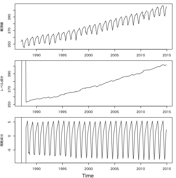
このモデルにより大気中の二酸化炭素濃度のデータを分析する。データの下調べは基礎から分かる時系列分析 1.時系列分析ひとめぐりで行っている。下調べより、このデータは全体的に右上がりの傾向が見られ、1ヶ月(1年に12周期)分の周期も認められる。
# ---
#  データの読み込み
# ---

Ryori = read.csv('co2_monthave_ryo.csv', fileEncoding = 'SJIS',
                 stringsAsFactors = FALSE)
y_all = ts(data = as.numeric(Ryori$二酸化炭素濃度の月平均値.綾里..ppm.),
           start = c(1987, 1), frequency = 12)
y     = window(y_all, end = c(2014, 12))

# ---
#  モデルの定義
# ---

build_dlm_CO2 = function(par){
  return(
    dlmModPoly(order = 2, dW = exp(par[1:2]), dV = exp(par[3])) +
    dlmModSeas(frequency = 12, dW = c(exp(par[4]), rep(0, times = 10)), dV = 0)
  )
}
4.2 パラメータの特定
システムノイズと観測ノイズを最尤推定する。
# ---
#  パラメータの特定
# ---

fit_dlm_CO2a = dlmMLE(y = y, parm = rep(0,4), build = build_dlm_CO2a)
mod          = build_dlm_CO2a(fit_dlm_CO2a$par)
4.3 フィルタリング
# ---
#  フィルタリング
# ---

dlmFiltered_obj = dlmFilter(y = y, mod = mod)

# フィルタ分布の平均、標準偏差の導出
m     = dropFirst(dlmFiltered_obj$m[,1]) # レベル成分
gamma = dropFirst(dlmFiltered_obj$m[,3]) # 周期成分

# 結果のプロット
oldpar = par(no.readonly = T)
par(mfrow = c(3,1))
par(oma = c(2,0,0,0))
par(mar = c(2,4,1,1))
par(family = "HiraginoSans-W4")
ts.plot(y, ylab = '観測値')
ts.plot(m, ylab = 'レベル成分', ylim = c(350, 405))
ts.plot(gamma, ylab = '周期成分', ylim = c(-9,6))
mtext(text = 'Time', side = 1, line = 1, outer = TRUE)
par(oldpar)
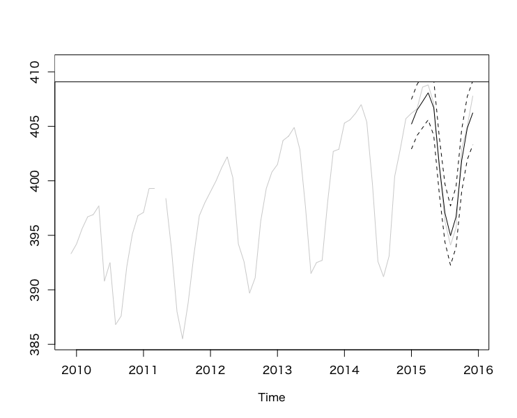
4.4予測
# ---
#  予測
# ---

dlmForecasted_object = dlmForecast(mod = dlmFiltered_obj, nAhead = 12)

# 予測分布の平均、標準偏差の導出
f_sd    = sqrt(as.numeric(dlmForecasted_object$Q))
f_lower = dlmForecasted_object$f + qnorm(0.025, sd = f_sd)
f_upper = dlmForecasted_object$f + qnorm(0.975, sd = f_sd)
y_all   = window(y_all, start = c(2009, 12), end = c(2015, 12))
y_union = ts.union(y_all, dlmForecasted_object$f, f_lower, f_upper)

# 結果のプロット
oldpar = par(no.readonly = T)
par(family = "HiraginoSans-W4")
ts.plot(y_union,
        col = c('lightgray', 'black', 'black', 'black'),
        lty = c('solid', 'solid', 'dashed', 'dashed'))
legend('bottomright',
       legend = c('観測値', '平均(予測分布)', '95%区間'),
       lty    = c('solid', 'solid', 'dashed', 'dashed'),
       col    = c('lightgray', 'black', 'black', 'black'),
       x      = 'topright', text.width = 26, cex = 0.6)
par(oldpar)