#Pythonで学ぶ制御工学< 状態空間モデルの時間応答 >
はじめに
基本的な制御工学をPythonで実装し,復習も兼ねて制御工学への理解をより深めることが目的である.
その第10弾として「状態空間モデルの時間応答」を扱う.
時間応答(状態空間モデルの時間応答)
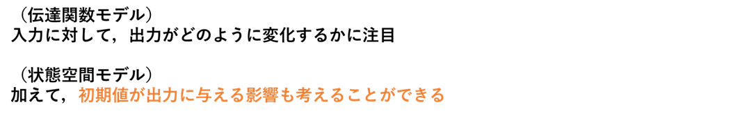
状態空間モデルと伝達関数モデルの時間応答との違いを,図を使っての説明を以下に示す.
続いて,状態空間モデルの時間応答について,図を使っての説明を以下に示す.

実装
ここでは,適当な状態空間モデルに対して,零入力応答・零状態応答(ステップ入力)・時間応答(ステップ入力)の図を出力する3つプログラムを実装する.
以下にソースコードとそのときの出力を示す.
ソースコード①:零入力応答
zero_input_response.py
"""
2021/03/02
@Yuya Shimizu

状態空間モデルの初期値応答
"""
import numpy as np
from control import  ss
from control.matlab import  initial
from for_plot import *
import matplotlib.pyplot as plt

## 状態空間モデルの設定
A = [[ 0,  1],
       [-4, -5]]

B = [[0],
        [1]]

C = [[ 1, 0],
       [ 0, 1]]     #np.eye(2)とも記述できる

D = [[0],
        [0]]        #np.zeros([2,1])とも記述できる

P = ss(A, B, C, D)


## 初期値応答
Td = np.arange(0, 5, 0.01)    #シミュレーション時間
x0 = [-0.3, 0.4]                    #初期値
x, t = initial(P, Td, x0)           #初期値応答(零入力応答)


## 描画
fig, ax = plt.subplots()
ax.plot(t, x[:, 0], label = '$x_1$')
ax.plot(t, x[:, 1], ls = '-.', label = '$x_2$')
ax.set_title('zero input response')
plot_set(ax, 't', 'x', 'best')
plt.show()
出力

ソースコード②:零状態応答(ステップ入力)
zero_state_response.py
"""
2021/03/02
@Yuya Shimizu

状態空間モデルの零状態応答
"""
import numpy as np
from control import  ss
from control.matlab import  step
from for_plot import *
import matplotlib.pyplot as plt

## 状態空間モデルの設定
A = [[ 0,  1],
       [-4, -5]]

B = [[0],
        [1]]

C = [[ 1, 0],
       [ 0, 1]]     #np.eye(2)とも記述できる

D = [[0],
        [0]]        #np.zeros([2,1])とも記述できる

P = ss(A, B, C, D)


## 零状態応答
Td = np.arange(0, 5, 0.01)    #シミュレーション時間
x, t = step(P, Td)           #零状態応答


## 描画
fig, ax = plt.subplots()
ax.plot(t, x[:, 0], label = '$x_1$')
ax.plot(t, x[:, 1], ls = '-.', label = '$x_2$')
ax.set_title('zero state response')
plot_set(ax, 't', 'x', 'best')
plt.show()
出力

ソースコード③:時間応答(ステップ入力)
time_response.py
"""
2021/03/02
@Yuya Shimizu

状態空間モデルの時間応答
"""
import numpy as np
from control import  ss
from control.matlab import  initial, step, lsim
from for_plot import *
import matplotlib.pyplot as plt

## 状態空間モデルの設定
A = [[ 0,  1],
       [-4, -5]]

B = [[0],
        [1]]

C = [[ 1, 0],
       [ 0, 1]]     #np.eye(2)とも記述できる

D = [[0],
        [0]]        #np.zeros([2,1])とも記述できる

P = ss(A, B, C, D)


## 時間応答 (=零入力応答 + 零状態応答)
Td = np.arange(0, 5, 0.01)    #シミュレーション時間
Ud = 1*(Td>0)
x0 = [-0.3, 0.4]            #初期値

xst, t = step(P, Td)           #零状態応答
xin, _ = initial(P, Td, x0)   #零入力応答
x, _, _ = lsim(P, Ud, Td, x0)   #時間応答

## 描画
fig, ax = plt.subplots(1, 2, figsize=(6, 2.3))

for i in [0, 1]:
    ax[i].plot(t, x[:, i], label = 'time response')             #時間応答の描画
    ax[i].plot(t, xst[:, i], ls = '--', label = 'zero state')    #零状態応答の描画
    ax[i].plot(t, xin[:, i], ls = '-.', label = 'zero input')    #零入力応答の描画

ax[0].set_title('response for $x_1$')
ax[1].set_title('response for $x_2$')
plot_set(ax[0], 't', '$x_1$')
plot_set(ax[1], 't', '$x_2$', 'best')
fig.tight_layout()
plt.show()
出力

零入力応答
ここで,零入力応答について,以前(https://qiita.com/Yuya-Shimizu/items/2e67581c13cfa3108809 )に示したアームを例に確認する.アームでは,初期角度と初期角速度を与えてスタートさせたとき,何も入力がなければ,粘性摩擦と重力の影響を受けて,最終的に鉛直下向きに垂れ下がった状態で静止する.つまり,時間が経過するにしたがって,0へ収束するということである.上で示した図からも分かる.
感想
式やグラフである制御対象の振る舞いを理解するというのは,直感的には難しいこともあるが,少しずつ慣れていきたい.入力応答や状態応答で解析する経験はなく,まだマスターできていないが,とりあえず基本的事項とPythonでの実装を学ぶことができた.
参考文献
Pyhtonによる制御工学入門 南 祐樹 著 オーム社