RBCモデル
- Real Business Cycle = 実物的景気循環
- 代表的家計を仮定
- 経済全体を 1つの家計に集約(個々の家計の異質性を無視)
- 技術進歩、生産性、嗜好などの実物的ショックが景気循環の要因
- 家計・企業は合理的期待のもとで最適に行動(効用最大化・利潤最大化)
- 更に経済事象を組み込んだDSGEモデル(Dynamic Stochastic General Equilibrium Model = 動学的確率的一般均衡モデル)は各国中央銀行や学界などが競って開発し活用
- 価格・賃金に摩擦あり
- 政策部門の存在
家計(効用最大化)
\begin{align}
\max_{\{c_t, l_t, k_{t+1}, h_{t+1}\}_{t=0}^{\infty}}
& \quad
E_t \sum_{t=0}^{\infty} \beta^t \, \xi_t
\left[
\frac{c_t^{1-\sigma}}{1-\sigma}
- \frac{\mu \, l_t^{1+\lambda}}{1+\lambda}
+ \psi \frac{(\theta_t \, h_t)^{1-\eta}}{1-\eta}
\right]
\\[2mm]
\text{s.t.} \quad
& c_t + q_t \, (h_{t+1} - (1-\delta_h) h_t) + k_{t+1} - (1-\delta_k) k_t
= w_t \, l_t + R_t \, (1-\theta_t) \, h_t + r_t \, k_t, \quad
\\[1mm]
\end{align}
企業(利潤最大化)
\begin{align}
\max_{\{k_t, l_t\}} \; \underbrace{\pi_t}_{\text{利潤}} \equiv \; & v_t k_t^{\alpha} l_t^{1-\alpha} - w_t l_t - r_t k_t \\[6pt]
\end{align}
内生変数
- ジャンプ変数
- $c_t$ :消費
- $l_t$ :労働供給
- $q_t$ :住宅価格
- 状態変数
- $k_t$ :物的資本ストック
- $h_t$ :住宅ストック
- 補助変数
- $\theta_t$ :持ち家率(自己使用住宅の比率)
- コード内ではジャンプ扱い可能(未来値が方程式に出るため)
- $r_t$ :物的資本のレンタル価格
- $w_t$ :賃金
- $R_t$ :賃貸住宅サービスの影の価格
- 賃貸市場がなくても(今回のモデル)住宅の非居住部分の価値を反映するための影の価格
- モデルを機能させるための技術・経済的な要素
- $\theta_t$ :持ち家率(自己使用住宅の比率)
外生変数
- 状態変数
- $v_t$ :技術ショック
- $\xi_t$ :嗜好ショック
- ショック
- $\varepsilon^v_t$ :技術ショックのイノベーション
- $\varepsilon^\xi_t$ :嗜好ショックのイノベーション
パラメータ
- $\beta \in (0,1)$ :割引因子
- $\sigma > 0$ :相対的リスク回避度
- $\mu > 0$ :労働の不効用の重み
- $\lambda > 0$ :逆フリッシュ弾力性
- $\psi > 0$ :住宅サービス効用ウェイト
- $\eta > 0$ :住宅サービス効用の曲率
- $\alpha \in (0,1)$ :資本分配率
- $\delta_k \in (0,1)$ :物的資本の減耗率
- $\delta_h \in (0,1)$ :住宅の減耗率
- $\phi \in (0,1)$ :技術ショックの自己相関
- $\rho_\xi \in (0,1)$ :嗜好ショックの自己相関
- $\theta^{ss} \in (0,1)$ :定常状態の持ち家率
- $\chi_q$ :住宅価格感応度
- $\chi_R$ :賃貸価格感応度
- $\chi_\xi$ :嗜好ショック感応度
家計の最適化問題の解法(制約付き最適化のためラグランジュ関数を定義 + 1階条件)
\begin{align}
\mathcal{L} = & \, E_t \sum_{t=0}^{\infty} \beta^t \, \xi_t \left[ \frac{c_t^{1-\sigma}}{1-\sigma} - \frac{\mu l_t^{1+\lambda}}{1+\lambda} + \psi \frac{(\theta_t h_t)^{1-\eta}}{1-\eta}  \right] \\
& + \sum_{t=0}^{\infty} \lambda_t \left[ w_t l_t + R_t (1-\theta_t) h_t + r_t k_t - c_t - q_t \left( h_{t+1} - (1-\delta_h) h_t \right) - k_{t+1} + (1-\delta_k) k_t \right] \\
\end{align}
\begin{align}
\frac{\partial \mathcal{L}}{\partial c_t}
= \beta^t\big(\xi_t c_t^{-\sigma} - \lambda_t\big) = 0
\quad\Rightarrow\quad
\lambda_t = \xi_t c_t^{-\sigma}
\end{align}
\begin{align}
\frac{\partial\mathcal{L}}{\partial l_t}
&=\beta^t\Big(-\xi_t\,\mu\,l_t^{\lambda}+\lambda_t\,w_t\Big)=0
\quad\Rightarrow\quad
\lambda_t\,w_t=\xi_t\,\mu\,l_t^{\lambda}
\end{align}
\begin{align}
\frac{\partial \mathcal{L}}{\partial k_{t+1}}
= -\beta^t \lambda_t
+ \beta^{t+1} E_t\!\big[\lambda_{t+1}(r_{t+1}+1-\delta_k)\big] = 0
\quad\Rightarrow\quad
\lambda_t = \beta E_t\!\big[\lambda_{t+1}(r_{t+1}+1-\delta_k)\big]
\end{align}
\begin{align}
\frac{\partial \mathcal{L}}{\partial h_{t+1}}
&=-\lambda_t\,q_t
\;+\;
\beta\,E_t\Big[
\xi_{t+1}\,\psi\,\frac{\partial}{\partial h_{t+1}}
\Big(\frac{(\theta_{t+1}h_{t+1})^{1-\eta}}{1-\eta}\Big)
+
\lambda_{t+1}\,R_{t+1}(1-\theta_{t+1})
+
\lambda_{t+1}\,q_{t+1}(1-\delta_h)
\Big]
=0
\quad\Rightarrow\quad
q_t
=
\beta\,\mathbb{E}_t\Big[
\frac{\lambda_{t+1}}{\lambda_t}
\Big\{R_{t+1}(1-\theta_{t+1}) + q_{t+1}(1-\delta_h)\Big\}
\;+\;
\frac{\xi_{t+1}}{\lambda_t}\,\psi\,\theta_{t+1}(\theta_{t+1}h_{t+1})^{-\eta}
\Big]
\end{align}
\begin{align}
\frac{\partial \mathcal{L}}{\partial \lambda_t}
=\beta^t\Big[
w_t\,l_t
+ R_t(1-\theta_t)\,h_t
+ r_t\,k_t
- c_t
- q_t\big(h_{t+1}-(1-\delta_h)h_t\big)
- k_{t+1}
+ (1-\delta_k)k_t
\Big]
=0
\quad\Rightarrow\quad
w_t\,l_t + R_t(1-\theta_t)\,h_t + r_t\,k_t
= c_t + q_t\big(h_{t+1}-(1-\delta_h)h_t\big) + k_{t+1} - (1-\delta_k)k_t
\end{align}
企業の最適化問題の解法(1階条件)
\begin{alignedat}{3}
\frac{\partial \pi_t}{\partial l_t} \; &=\; v_t(1-\alpha)\,k_t^{\alpha} l_t^{-\alpha} \;-\; w_t
\; &=\; 0 \; &\Rightarrow\; &\quad
w_t \; &=\; (1-\alpha)\, v_t\, k_t^{\alpha} l_t^{-\alpha}
\\[2pt]
\frac{\partial \pi_t}{\partial k_t} \; &=\; v_t \alpha\, k_t^{\alpha-1} l_t^{\,1-\alpha} \;-\; r_t
\; &=\; 0 \; &\Rightarrow\; &\quad
r_t \; &=\; \alpha\, v_t\, k_t^{\alpha-1} l_t^{\,1-\alpha}
\end{alignedat}
非線形経済システム(家計・企業のFirst Order Condition(1階条件) + 補助条件 + アドホックルール + AutoRegression(1)より)
\begin{alignat}{2}
m_{t+1} \; \equiv \;& \frac{\xi_{t+1}\,c_{t+1}^{-\sigma}}{\xi_t\,c_t^{-\sigma}}
\end{alignat}
\begin{alignat}{2}\
R_t \; \equiv \;& \psi\,\big((1-\theta_t)h_t\big)^{-\eta}\,c_t^{\sigma}
\end{alignat}
\begin{alignat}{2}
\xi_t\,c_t^{-\sigma} \;&=\;&
\beta\,E_t\!\left[
  \xi_{t+1}\,c_{t+1}^{-\sigma}\,\Big(1-\delta_k + \alpha\,v_{t+1}\,k_{t+1}^{\alpha-1}l_{t+1}^{\,1-\alpha}\Big)
\right]
\tag{1}
\end{alignat}
\begin{alignat}{3}
\mu\,l_t^{\lambda} \;&=\;& c_t^{-\sigma}\,(1-\alpha)\,v_t\,k_t^{\alpha}l_t^{-\alpha}
\tag{2}
\end{alignat}
\begin{alignat}{2}

q_t \;&=\;&
\beta E_t \left[ m_{t+1} \left( (1-\delta_h) q_{t+1} + R_{t+1}(1-\theta_{t+1}) \right) \right]
+ \beta E_t \left[ m_{t+1} \psi \theta_{t+1} (\theta_{t+1} h_{t+1})^{-\eta} c_{t+1}^\sigma \right]

\tag{3}
\end{alignat}
\begin{alignat}{2}
\psi\,(\theta_t h_t)^{-\eta} \;&=\;& q_t\,c_t^{-\sigma}
\tag{4}
\end{alignat}
\begin{alignat}{2}
w_t\,l_t \;+\; R_t\,(1-\theta_t)\,h_t \;+\; r_t\,k_t
\;=\;
c_t \;+\; q_t\bigl(h_{t+1}-(1-\delta_h)h_t\bigr)
\;+\; k_{t+1} \;-\; (1-\delta_k)k_t
\tag{5}
\end{alignat}
\begin{alignat}{2}
\theta_t-\theta^{ss} \;&=\;&
-\,\chi_Q\,(q_t-q^{ss}) \;+\; \chi_R\,(R_t-R^{ss}) \;+\; \chi_\xi\,(\xi_t-\xi^{ss})
\tag{6}
\end{alignat}
\begin{alignat}{2}
v_{t+1} \;&=\;& \phi\,v_t + \varepsilon_t^{\,v}
\tag{7}
\end{alignat}
\begin{alignat}{2}
\xi_{t+1} \;&=\;& \rho_{\xi}\,\xi_t + \varepsilon_t^{\,\xi}
\tag{8}
\end{alignat}
- (1) 資本のオイラー方程式(FOCより)
- (2) 労働の一階条件式(FOCより)
- (3) 住宅価格のオイラー方程式(FOCより)
- (4) 住宅サービスと消費の限界代替率(補助条件)
- 補助条件: ラグランジュのFOCから直接は出ないが、モデルの均衡を閉じるために必要な追加条件
- (5) 財市場の資源制約(FOCより)
- (6) 住宅利用率(アドホックルール)
- (7) 技術ショック過程(AR(1))
- (8) 嗜好ショック過程(AR(1))
コード
python
# --- coding: utf-8 ---
import numpy as np
from scipy.linalg import ordqz
import matplotlib.pyplot as plt
# -------------------------------------------------
# Numerical Jacobian (central differences)
# -------------------------------------------------
def numerical_jacobian(func, x0, eps=1e-6):
"""
Compute a central-difference Jacobian J of func at x0.
func: R^n -> R^m, returns a vector residual
J: (m x n) matrix of partial derivatives
"""
x0 = np.asarray(x0, float)
f0 = np.asarray(func(x0))
m, n = f0.size, x0.size
J = np.zeros((m, n))
h = eps * (1 + np.abs(x0))
for j in range(n):
x1 = x0.copy(); x1[j] += h[j]
x2 = x0.copy(); x2[j] -= h[j]
f1 = np.asarray(func(x1))
f2 = np.asarray(func(x2))
J[:, j] = (f1 - f2) / (2 * h[j])
return J
# -------------------------------------------------
# Residual builder: bind names -> vector-valued function
# -------------------------------------------------
def make_residual_function(varnames, shock_names, residual_eqs):
"""
Build a residual function F(x, params) from named variables and equations.
x packs [future vars, current vars, shocks]
"""
def residual(x, params):
X = {name: x[i] for i, name in enumerate(varnames + shock_names)}
return np.array([eq(X, params) for eq in residual_eqs])
return residual
# -------------------------------------------------
# QZ solver with BK check (ordqz(C, B))
# -------------------------------------------------
def solve_qz_system(B, C, njump, npred, D=None, verbose=False):
"""
Solve B x_{t+1} + C x_t + D eps_t = 0 via generalized Schur (QZ).
Ordering uses ordqz(C, B) so eigenvalues are lambda = alpha/beta of (C - lambda B).
BK condition: number of unstable roots must equal njump.
Returns policy P (jump = P state), transition A (state), shock map G.
"""
def sort_unstable(alpha, beta):
# Mark eigenvalues outside unit circle as "unstable"
tol = 1e-12
alpha = np.asarray(alpha)
beta = np.asarray(beta)
mask_zero_beta = np.abs(beta) < tol
lam_abs = np.zeros_like(alpha, float)
lam_abs[mask_zero_beta] = np.inf
lam_abs[~mask_zero_beta] = np.abs(alpha[~mask_zero_beta] / beta[~mask_zero_beta])
return lam_abs > 1.0
# Run QZ with reordering by custom callable
res = ordqz(C, B, sort=sort_unstable, output="real")
# Handle SciPy return formats (object or tuple)
if hasattr(res, "AA"):
AA = res.AA; BB = res.BB; alpha = res.alpha; beta = res.beta; Q = res.Q; Z = res.Z
else:
seq = list(res)
if len(seq) == 6:
AA, BB, alpha, beta, Q, Z = seq
elif len(seq) == 4:
AA, BB, Q, Z = seq
alpha = np.diag(AA); beta = np.diag(BB)
else:
raise RuntimeError(f"Unexpected ordqz output length {len(seq)}")
lam = np.array(alpha) / np.array(beta)
mask_unstable = np.abs(lam) > 1.0
nunstable = int(mask_unstable.sum())
if verbose:
print("QZ generalized eigenvalues:", lam)
print("Unstable roots:", nunstable, "Jump vars:", njump)
if nunstable != njump:
raise RuntimeError(f"Blanchard-Kahn failed: unstable roots={nunstable} != jump vars={njump}")
# Stable invariant subspace (right Schur vectors)
Z_stable = Z[:, ~mask_unstable]
# Variable ordering: [jump | state] after grouping
jump_idx = list(range(njump)) # first njump rows
state_idx = list(range(njump, njump+npred)) # next npred rows
# Policy: jump = P * state
ZJ = Z_stable[jump_idx, :]
ZS = Z_stable[state_idx, :]
P = (np.linalg.solve(ZS.T, ZJ.T)).T
# State transition A on the stable block
idx_stable = np.where(~mask_unstable)[0]
AA22 = AA[np.ix_(idx_stable, idx_stable)]
BB22 = BB[np.ix_(idx_stable, idx_stable)]
A_schur = np.linalg.solve(BB22, AA22)
A = ZS @ A_schur @ np.linalg.inv(ZS)
# Shock map G
if D is None:
G = np.zeros((npred, 1))
else:
D_q = Q.T @ D # left transform to QZ coordinates
D2 = D_q[idx_stable, :] # keep stable rows
G_schur = np.linalg.solve(BB22, D2)
G = ZS @ G_schur
return P.real, A.real, G.real, lam.real
# -------------------------------------------------
# Linear simulation: state and jump paths
# -------------------------------------------------
def simulate_system(A, G, P, T, shock_process, x_state0=None):
"""
Simulate linear system:
state_{t+1} = A state_t + G eps_t
jump_t = P state_t
"""
nstate = A.shape[0]
njump = P.shape[0]
x_state = np.zeros(nstate) if x_state0 is None else np.asarray(x_state0, float)
state_path = np.zeros((T+1, nstate))
jump_path = np.zeros((T+1, njump))
state_path[0] = x_state
jump_path[0] = P @ x_state
for t in range(T):
eps = shock_process(t) if shock_process is not None else np.zeros(G.shape[1])
x_next = A @ x_state + G @ eps
state_path[t+1] = x_next
jump_path[t+1] = P @ x_next
x_state = x_next
return state_path, jump_path
# -------------------------------------------------
# Build model: steady state, residuals, Jacobian, blocks
# -------------------------------------------------
def build_model(params):
def rental(theta, h, c, p):
"""Shadow rental price: R = psi * ((1 - theta) * h)^(-eta) * c^(sigma)."""
return p["psi"] * (((1.0 - theta) * h) ** (-p["eta"])) * (c ** p["sigma"])
def ss_vals(p):
v = 1.0; xi = 1.0; theta = p["theta_ss"]
kls = (((1/p["beta"]) + p["delta_k"] - 1) / p["alpha"])**(1/(p["alpha"]-1))
w = (1-p["alpha"]) * kls**p["alpha"]
cl = kls**p["alpha"] - p["delta_k"]*kls
l = ((w/p["mu"]) * (cl**(-p["sigma"])) * xi)**(1/(p["lamda"]+p["sigma"])) # (kept as-is for now)
k = l*kls
c = l*cl
h = ((p["psi"]*(1-p["beta"]))/(p["beta"]*(1-p["delta_h"])))**(1/p["eta"]) * c**(p["sigma"]/p["eta"])
q = (p["beta"] * p["psi"] * xi * (theta*h)**(-p["eta"])) / (1 - p["beta"] * (1 - p["delta_h"]))
R = p["psi"] * ((1.0 - theta) * h)**(-p["eta"]) * (c**(p["sigma"]))
return dict(l=l, c=c, k=k, h=h, q=q, R=R, v=v, xi=xi, theta=theta)
ss = ss_vals(params)
# --- REORDER to [jump | state] in BOTH future & current ---
future_vars = ["l_f","c_f","q_f","theta_f","k_f","h_f","v_f","xi_f"]
current_vars = ["l","c","q","theta","k","h","v","xi"]
shock_vars = ["eps_v","eps_xi"]
varnames = future_vars + current_vars
# Equations
def eq1(X,p):
mpk_f = p["alpha"]*X["k_f"]**(p["alpha"]-1) * X["l_f"]**(1-p["alpha"]) * X["v_f"]
return X["xi"]*X["c"]**(-p["sigma"]) - p["beta"]*X["xi_f"]*X["c_f"]**(-p["sigma"]) * (1-p["delta_k"] + mpk_f)
def eq2(X,p):
"""Labor FOC: -mu l_t^{lamda} + c_t^{-sigma} w_t = 0 (xi cancels)"""
w_t = (1 - p["alpha"]) * X["k"]**p["alpha"] * X["l"]**(-p["alpha"]) * X["v"]
return -p["mu"] * X["l"]**p["lamda"] + X["c"]**(-p["sigma"]) * w_t
def eq3(X, p):
"""
Budget/resource constraint at time t with rental income:
y_t + R_t * (1 - theta_t) * h_t
= c_t + q_t * (h_{t+1} - (1 - delta_h) * h_t) + k_{t+1} - (1 - delta_k) * k_t
where y_t = v_t * k_t^alpha * l_t^(1 - alpha),
R_t = psi * (((1 - theta_t) * h_t)^(-eta)) * c_t^(sigma).
"""
# Output (competitive firm ⇒ w_t l_t + r_t k_t = y_t)
y = (X["k"] ** p["alpha"]) * (X["l"] ** (1 - p["alpha"])) * X["v"]
# Current-period rental price and income
R_cur = p["psi"] * (((1.0 - X["theta"]) * X["h"]) ** (-p["eta"])) * (X["c"] ** p["sigma"])
# Residual of the budget/resource constraint
return (
y + R_cur * (1.0 - X["theta"]) * X["h"]
- X["c"]
- X["q"] * (X["h_f"] - (1.0 - p["delta_h"]) * X["h"])
- X["k_f"] + (1.0 - p["delta_k"]) * X["k"]
)
def eq4(X, p):
"""
Housing Euler with explicit rental term (theta is rule-based, not a choice).
q_t = beta * m_{t+1} * {
R_{t+1}*(1 - theta_{t+1})
+ (1 - delta_h) * q_{t+1}
+ psi * c_{t+1}^{sigma} * theta_{t+1} * (theta_{t+1}*h_{t+1})^{-eta}
}
where m_{t+1} = (xi_{t+1} * c_{t+1}^{-sigma}) / (xi_t * c_t^{-sigma}).
"""
# SDF ratio m = lambda_{t+1} / lambda_t
m = (X["xi_f"] * X["c_f"]**(-p["sigma"])) / (X["xi"] * X["c"]**(-p["sigma"]))
R_f = rental(X["theta_f"], X["h_f"], X["c_f"], p)
term_rental = m * R_f * (1.0 - X["theta_f"]) # R_{t+1}*(1 - theta_{t+1})
term_survival = m * (1.0 - p["delta_h"]) * X["q_f"] # (1 - delta_h) * q_{t+1}
term_ownuse = (m * (X["c_f"] ** p["sigma"]) * p["psi"] * X["theta_f"] * (X["theta_f"] * X["h_f"]) ** (-p["eta"])) # own-use marginal utility
return X["q"] - p["beta"] * (term_rental + term_survival + term_ownuse)
def eq5(X,p):
return X["v_f"] - p["phi"] * X["v"] - X["eps_v"]
def eq6(X,p):
return X["xi_f"] - p["rho_xi"] * X["xi"] - X["eps_xi"]
def eq7(X,p):
"""Auxiliary intratemporal: psi (theta h)^{-eta} = q c^{-sigma}"""
return p["psi"] * (X["theta"] * X["h"])**(-p["eta"]) - X["q"] * X["c"]**(-p["sigma"])
def eq8(X,p):
"""Theta reaction rule using shadow rental price R_t."""
R_cur = rental(X["theta"], X["h"], X["c"], p)
return (X["theta"] - p["theta_ss"]) \
- p["chi_q"] * (X["q"] - ss["q"]) \
+ p["chi_R"] * (R_cur - ss["R"]) \
residual_eqs = [eq1, eq2, eq3, eq4, eq5, eq6, eq7, eq8]
residual = make_residual_function(varnames, shock_vars, residual_eqs)
# Steady-state vector consistent with new ordering
xss = np.array([
ss["l"], ss["c"], ss["q"], ss["theta"], ss["k"], ss["h"], ss["v"], ss["xi"],
ss["l"], ss["c"], ss["q"], ss["theta"], ss["k"], ss["h"], ss["v"], ss["xi"],
0.0, 0.0
], float)
# Jacobian
J = numerical_jacobian(lambda x: residual(x, params), xss)
J_fc = J[:, :16]
# Column scaling (future/current each length-8, same ordering)
scale_f = np.array([ss["l"], ss["c"], ss["q"], ss["theta"], ss["k"], ss["h"], ss["v"], ss["xi"]])
scale_c = np.array([ss["l"], ss["c"], ss["q"], ss["theta"], ss["k"], ss["h"], ss["v"], ss["xi"]])
TW_f = np.tile(scale_f, (len(residual_eqs), 1))
TW_c = np.tile(scale_c, (len(residual_eqs), 1))
B = -J_fc[:, :8] * TW_f
C = J_fc[:, 8:16] * TW_c
D_raw = J[:, -2:]
D = D_raw * np.array([ss["v"], ss["xi"]])
return B, C, D, ss
# -------------------------------------------------
# Top-level solve wrapper
# -------------------------------------------------
def try_solve(params, verbose=False):
"""
Build model and solve QZ with BK check. Expect njump=4 (l,c,q,theta), npred=4 (k,h,v,xi).
"""
B, C, D, ss = build_model(params)
if verbose:
print("Shapes -> B:", B.shape, "C:", C.shape, "D:", D.shape)
P, A, G, lam = solve_qz_system(B, C, njump=4, npred=4, D=D, verbose=verbose)
return (P, A, G, lam), ss
# -------------------------------------------------
# Single-figure IRF grid (one image with subplots)
# -------------------------------------------------
def save_irfs_grid(prefix, state_path, jump_path, ss, params):
"""
Create one figure with multiple subplots, similar to the provided screenshot.
Plots: theta, h, q, R, c, l, k (7 panels). Saved as f"{prefix}_irfs_grid.png".
"""
# Recompute level series (same as save_irfs)
k_hat = state_path[:,0]
h_hat = state_path[:,1]
v_hat = state_path[:,2]
xi_hat = state_path[:,3]
l_hat = jump_path[:,0]
c_hat = jump_path[:,1]
q_hat = jump_path[:,2]
theta_hat = jump_path[:,3]
k_lev = ss["k"] * (1.0 + k_hat)
h_lev = ss["h"] * (1.0 + h_hat)
v_lev = ss["v"] * (1.0 + v_hat)
xi_lev = ss["xi"] * (1.0 + xi_hat)
l_lev = ss["l"] * (1.0 + l_hat)
c_lev = ss["c"] * (1.0 + c_hat)
q_lev = ss["q"] * (1.0 + q_hat)
theta_lev = np.clip(ss["theta"] * (1.0 + theta_hat), 1e-8, 1.0 - 1e-8)
psi = params["psi"]
eta = params["eta"]
sigma = params["sigma"]
R_lev = psi * ((1.0 - theta_lev) * h_lev)**(-eta) * (np.maximum(1e-12, c_lev)**(sigma))
# Deviations (percentage)
theta_hat_pct = (theta_lev / ss["theta"]) - 1.0
h_hat_pct = (h_lev / ss["h"]) - 1.0
q_hat_pct = (q_lev / ss["q"]) - 1.0
R_hat = (R_lev / ss["R"]) - 1.0
c_hat_pct = (c_lev / ss["c"]) - 1.0
l_hat_pct = (l_lev / ss["l"]) - 1.0
k_hat_pct = (k_lev / ss["k"]) - 1.0
t = np.arange(len(k_hat_pct))
import matplotlib.pyplot as plt
fig, axes = plt.subplots(3, 3, figsize=(10, 8))
fig.suptitle(f"IRFs - {prefix}", fontsize=14)
# Top row
axes[0,0].plot(t, theta_hat_pct); axes[0,0].set_title("Homeownership (θ)"); axes[0,0].grid(True)
axes[0,1].plot(t, h_hat_pct); axes[0,1].set_title("Housing stock (h)"); axes[0,1].grid(True)
axes[0,2].plot(t, q_hat_pct); axes[0,2].set_title("House price (q)"); axes[0,2].grid(True)
# Middle row
axes[1,0].plot(t, R_hat); axes[1,0].set_title("Rent (R)"); axes[1,0].grid(True)
axes[1,1].plot(t, c_hat_pct); axes[1,1].set_title("Consumption (c)"); axes[1,1].grid(True)
axes[1,2].plot(t, l_hat_pct); axes[1,2].set_title("Labor (l)"); axes[1,2].grid(True)
# Bottom row
axes[2,0].plot(t, k_hat_pct); axes[2,0].set_title("Capital (k)"); axes[2,0].grid(True)
axes[2,1].axis('off'); axes[2,2].axis('off')
plt.tight_layout(rect=[0, 0.03, 1, 0.95])
plt.savefig(prefix + "_irfs_grid.png", dpi=150)
# -------------------------------------------------
# IRF simulation (unit shock at t=0)
# -------------------------------------------------
def simulate_irf(A, G, P, T, amp, shock):
"""
Produce an IRF for either preference ('pref') or technology ('tech') shock.
eps = [eps_v, eps_xi], with a unit shock in selected dimension at t=0.
"""
if shock=="pref":
def shock_process(t): return np.array([0.0, amp if t==0 else 0.0])
else:
def shock_process(t): return np.array([amp if t==0 else 0.0, 0.0])
state_path, jump_path = simulate_system(A, G, P, T, shock_process)
return state_path, jump_path
def simulate_with_eps_series(A, G, P, eps_series, x_state0=None):
T = eps_series.shape[0]
nstate = A.shape[0]
njump = P.shape[0]
x_state = np.zeros(nstate) if x_state0 is None else np.asarray(x_state0, float)
state_path = np.zeros((T+1, nstate))
jump_path = np.zeros((T+1, njump))
state_path[0] = x_state
jump_path[0] = P @ x_state
for t in range(T):
eps = eps_series[t]
x_next = A @ x_state + G @ eps
state_path[t+1] = x_next
jump_path[t+1] = P @ x_next
x_state = x_next
return state_path, jump_path
def _extract_hats(state_path, jump_path):
k_hat = state_path[:,0]; h_hat = state_path[:,1]
v_hat = state_path[:,2]; xi_hat = state_path[:,3]
l_hat = jump_path[:,0]; c_hat = jump_path[:,1]
q_hat = jump_path[:,2]; theta_hat = jump_path[:,3]
return {
'theta': theta_hat,
'h': h_hat, 'q': q_hat,
'c': c_hat, 'l': l_hat,
'k': k_hat,
'v': v_hat, 'xi': xi_hat
}
def compute_historical_decomposition(A, G, P, ss, params, eps_series):
T, nshock = eps_series.shape
contrib = {}
for i in range(nshock):
eps_i = np.zeros_like(eps_series)
eps_i[:, i] = eps_series[:, i]
sp_i, jp_i = simulate_with_eps_series(A, G, P, eps_i)
hats_i = _extract_hats(sp_i, jp_i)
if i == 0:
for k in hats_i.keys():
contrib[k] = np.zeros((nshock, hats_i[k].shape[0]))
for k, series in hats_i.items():
contrib[k][i, :] = series
sigma = params['sigma']; eta = params['eta']; theta_ss = ss['theta']
R_contrib = np.zeros((nshock, T+1))
for i in range(nshock):
c_i = contrib['c'][i]
h_i = contrib['h'][i]
theta_i = contrib['theta'][i]
R_contrib[i] = sigma * c_i - eta * h_i + eta * (theta_ss/(1.0 - theta_ss)) * theta_i
contrib['R'] = R_contrib
return contrib
def compute_fevd_from_hist(contrib, var_list):
fevd = {}
for v in var_list:
X = contrib[v] # (nshock, T+1)
total = X.sum(axis=0)
var_total = total.var(ddof=0) + 1e-12
shares = X.var(axis=1, ddof=0) / var_total
ssum = shares.sum()
if ssum > 0:
shares = shares / ssum
fevd[v] = shares
return fevd
def save_fevd_figure(prefix, fevd, vars_plot, shock_names):
"""
FEVD (variance decomposition) as a single image (English).
Auto-adjust rows/columns so labels fit (increase rows if needed).
Output: f"{prefix}_summary.png"
"""
import numpy as np
import matplotlib.pyplot as plt
from math import ceil
titles = {
'theta': 'Homeownership (θ)',
'h': 'Housing Stock (h)',
'q': 'House Price (q)',
'R': 'Shadow Rent (R)',
'c': 'Consumption (c)',
'l': 'Labor (l)',
'k': 'Capital (k)'
}
nvars = len(vars_plot)
nshock = len(shock_names)
# ---------- Adaptive grid ----------
if nvars >= 9:
ncols = 2
elif nvars >= 7:
ncols = 3
else:
ncols = min(4, nvars)
nrows = ceil(nvars / ncols)
width_per_panel = 3.8 if ncols >= 3 else 4.5
height_per_panel = 3.2
fig_w = max(12, width_per_panel * ncols)
fig_h = max(4.5, height_per_panel * nrows)
fig, axes = plt.subplots(nrows, ncols, figsize=(fig_w, fig_h), constrained_layout=True)
if nrows == 1 and ncols == 1:
axes = np.array([[axes]])
elif nrows == 1:
axes = np.array([axes])
fig.suptitle("Variance Decomposition (FEVD, %)", fontsize=12, y=0.995)
colors = ['tab:blue', 'tab:orange', 'tab:green', 'tab:red']
panel_idx = 0
for r in range(nrows):
for c in range(ncols):
ax = axes[r, c]
if panel_idx < nvars:
v = vars_plot[panel_idx]
shares = fevd[v] # shape (nshock,)
ax.bar(range(nshock), shares * 100.0, color=colors[:nshock])
ax.set_xticks(range(nshock))
# Short shock labels to reduce width
# If needed, pass already-short labels from _run_decompositions (e.g., ['Tech (v)','Pref (xi)'])
ax.set_xticklabels(shock_names, fontsize=9)
ax.set_title(titles.get(v, v), fontsize=11)
ax.set_ylim(0, 100)
ax.grid(True, axis='y', alpha=0.3)
else:
ax.axis('off')
panel_idx += 1
try:
plt.tight_layout(pad=0.6, w_pad=0.8, h_pad=0.6)
except Exception:
plt.tight_layout()
out = f"{prefix}_summary.png"
plt.savefig(out, dpi=150)
return out
def save_hist_figure(prefix, contrib, T, vars_plot, shock_names):
"""
Historical Decomposition as a single image (English).
Auto-adjust rows/columns so labels fit (increase rows if needed).
Output: f"{prefix}_summary.png"
"""
import numpy as np
import matplotlib.pyplot as plt
from math import ceil
# Short English titles per variable (panel titles only show variable)
titles = {
'theta': 'Homeownership (θ)',
'h': 'Housing Stock (h)',
'q': 'House Price (q)',
'R': 'Shadow Rent (R)',
'c': 'Consumption (c)',
'l': 'Labor (l)',
'k': 'Capital (k)'
}
colors = ['tab:blue', 'tab:orange', 'tab:green', 'tab:red']
nvars = len(vars_plot)
tgrid = np.arange(T + 1)
# ---------- Adaptive grid ----------
# Start with up to 4 columns; if titles seem long, cap at 3 or 2 to give more width.
# Heuristic: for 7+ variables use 3 cols; for 9+ use 2 cols.
if nvars >= 9:
ncols = 2
elif nvars >= 7:
ncols = 3
else:
ncols = min(4, nvars)
nrows = ceil(nvars / ncols)
# ---------- Figure size ----------
# Wider panels reduce title truncation. Tune per-panel width/height here.
width_per_panel = 3.8 if ncols >= 3 else 4.5
height_per_panel = 3.4
fig_w = max(12, width_per_panel * ncols)
fig_h = max(6, height_per_panel * nrows)
fig, axes = plt.subplots(nrows, ncols, figsize=(fig_w, fig_h), constrained_layout=True)
# Normalize axes to 2D array
if nrows == 1 and ncols == 1:
axes = np.array([[axes]])
elif nrows == 1:
axes = np.array([axes])
# Global subtitle (keeps panel titles short)
fig.suptitle("Historical Decomposition (hat)", fontsize=12, y=0.995)
# ---------- Draw panels ----------
idx = 0
for r in range(nrows):
for c in range(ncols):
ax = axes[r, c]
if idx < nvars:
v = vars_plot[idx]
S = contrib[v] # (nshock, T+1)
ax.stackplot(tgrid, *S, colors=colors[:S.shape[0]], labels=shock_names)
ax.plot(tgrid, S.sum(axis=0), color='k', lw=1.2, label='Total')
ax.set_title(titles.get(v, v), fontsize=11)
ax.grid(True, alpha=0.3)
# Show legend only once to save space
if idx == 0:
ax.legend(loc='upper right', fontsize=8)
else:
ax.axis('off')
idx += 1
# Extra tightening of layout (padding & spacing)
try:
plt.tight_layout(pad=0.6, w_pad=0.8, h_pad=0.8)
except Exception:
plt.tight_layout()
out = f"{prefix}_summary.png"
plt.savefig(out, dpi=150)
return out
def _run_decompositions(A, G, P, ss, params, seed=42, T=120, shock_scale=0.01):
rng = np.random.default_rng(seed)
eps_series = rng.standard_normal((T, 2)) * shock_scale # [eps_v, eps_xi]
contrib = compute_historical_decomposition(A, G, P, ss, params, eps_series)
vars_plot = ['theta','h','q','R','c','l','k']
fevd = compute_fevd_from_hist(contrib, vars_plot)
shock_names = ['tech (v)', 'pref (xi)']
f1 = save_fevd_figure('fevd', fevd, vars_plot, shock_names)
f2 = save_hist_figure('hist', contrib, T, vars_plot, shock_names)
print(f"saved FEVD: {f1}")
print(f"saved historical decomposition: {f2}")
def _matrix_power_iter(A, H):
"""Yield A^h for h = 0..H-1 by iterative multiplication (fast & stable)."""
n = A.shape[0]
M = np.eye(n)
for h in range(H):
yield M
M = A @ M
def compute_fevd_rigorous_with_rent(
A, G, P, ss, params, H=20, Omega=None, orthogonalize=True,
var_names_jump=('l','c','q','theta'),
var_names_state=('k','h','v','xi'),
include_rent=True
):
"""
Compute rigorous FEVD for both jump and state variables using
M = [P; I_nstate], optionally adding a log-linearized shadow rent row.
Parameters
----------
A, G, P : np.ndarray
Linearized system matrices with y_t = P x_t (jump from states).
ss : dict
Steady-state dictionary, must contain 'theta'.
params : dict
Model parameters, must contain 'sigma' and 'eta'.
H : int
Forecast horizon (# of steps ahead) for FEVD accumulation.
Omega : (nshock x nshock) covariance
Shock covariance; identity if None.
orthogonalize : bool
If True, orthogonalize shocks via Cholesky/eigen so covariance is I.
var_names_jump : tuple[str]
Names in jump ordering consistent with rows of P. Default ('l','c','q','theta').
var_names_state : tuple[str]
Names of state variables consistent with columns of A. Default ('k','h','v','xi').
include_rent : bool
If True, append one extra measurement row m_R representing shadow rent.
Returns
-------
fevd : dict[str -> np.ndarray]
For each variable name in jump + state (+ 'R' if include_rent),
returns a (nshock,) array of FEVD shares summing to 1.
"""
nstate = A.shape[0]
njump = P.shape[0]
nshock = G.shape[1]
# Base measurement: jump + state
M = np.vstack([P, np.eye(nstate)]) # (njump + nstate) x nstate
names_all = list(var_names_jump) + list(var_names_state)
# Optionally add shadow rent (R) measurement row using log-linear coefficients
if include_rent:
sigma = float(params['sigma'])
eta = float(params['eta'])
theta_ss = float(ss['theta'])
# Indices in jump ordering: ('l','c','q','theta') -> c_idx = 1, theta_idx = 3
c_idx = var_names_jump.index('c')
theta_idx = var_names_jump.index('theta')
# Index in state ordering: ('k','h','v','xi') -> h_idx = 1
h_idx = var_names_state.index('h')
# Unit row picking the housing state
e_h_row = np.zeros(nstate)
e_h_row[h_idx] = 1.0
# m_R maps states to R_hat using: R_hat ≈ σ c_hat − η h_hat + η*(θ_ss/(1 − θ_ss)) θ_hat
m_R = sigma * P[c_idx, :] \
- eta * e_h_row \
+ eta * (theta_ss / (1.0 - theta_ss)) * P[theta_idx, :]
M = np.vstack([M, m_R[None, :]]) # append as last row
names_all.append('R')
# Shock covariance and orthogonalization
if Omega is None:
Omega = np.eye(nshock)
Omega = np.asarray(Omega, float)
if orthogonalize:
try:
L = np.linalg.cholesky(Omega)
except np.linalg.LinAlgError:
# Fallback to eigen factor for PSD covariance
eigvals, eigvecs = np.linalg.eigh(Omega)
eigvals = np.clip(eigvals, 0.0, None)
L = eigvecs @ np.diag(np.sqrt(eigvals))
Gt = G @ L
W = np.eye(nshock)
else:
Gt = G.copy()
W = Omega
# Accumulate IRFs over horizons: C_h = M A^h G_tilde
C_list = []
for Ah in _matrix_power_iter(A, H):
C_h = M @ Ah @ Gt # (nvars_total x nshock)
C_list.append(C_h)
# Total FE variance and per-shock contributions
nvars_total = M.shape[0]
total_var = np.zeros(nvars_total)
contrib = np.zeros((nvars_total, nshock))
for C_h in C_list:
if np.allclose(W, np.eye(nshock)):
total_var += (C_h**2).sum(axis=1) # row-wise sum of squares
contrib += (C_h**2) # per-shock column squares
else:
total_var += np.einsum('ij,jk,ik->i', C_h, W, C_h)
contrib += C_h @ W * C_h # elementwise product
# Normalize to shares
fevd = {}
eps = 1e-12
for j, name in enumerate(names_all):
s = contrib[j, :] / (total_var[j] + eps)
ssum = s.sum()
if ssum > 0:
s = s / ssum
fevd[name] = s
return fevd
def save_fevd_rigorous_figure(prefix, fevd_shares, vars_plot, shock_names):
"""
Save a single FEVD image (bar charts, % shares) in a fixed 3x3 grid.
If fewer than 9 panels are provided, remaining cells are hidden.
If more than 9 are provided, only the first 9 are plotted.
Parameters
----------
prefix : str
Output file prefix (image will be f"{prefix}_summary.png").
fevd_shares : dict[str -> np.ndarray]
For each variable name, a 1D array of shares (nshock,), summing to 1.
vars_plot : list[str]
Variable names (order of panels). Will be truncated/padded to 9.
shock_names : list[str]
Short labels for shocks (e.g., ['Tech (v)', 'Pref (xi)']).
"""
import numpy as np
import matplotlib.pyplot as plt
titles = {
'theta': 'Homeownership (θ)',
'h': 'Housing Stock (h)',
'q': 'House Price (q)',
'R': 'Shadow Rent (R)',
'c': 'Consumption (c)',
'l': 'Labor (l)',
'k': 'Capital (k)',
'v': 'Technology state (v)',
'xi': 'Preference state (xi)'
}
colors = ['tab:blue', 'tab:orange', 'tab:green', 'tab:red']
# --- Fix the panel grid to 3 x 3 ---
nrows, ncols = 3, 3
max_panels = nrows * ncols
# Prepare panel list (first 9 only); pad with None if shorter
vars_plot = list(vars_plot[:max_panels])
if len(vars_plot) < max_panels:
vars_plot += [None] * (max_panels - len(vars_plot))
# --- Figure size tuned for text to fit in 3x3 ---
width_per_panel = 3.8 # increase to 4.2 if labels overflow
height_per_panel = 3.2 # increase to 3.5 if labels overflow
fig_w = width_per_panel * ncols
fig_h = height_per_panel * nrows
fig, axes = plt.subplots(nrows, ncols, figsize=(fig_w, fig_h), constrained_layout=True)
fig.suptitle("Variance Decomposition (FEVD, orthogonalized shocks)", fontsize=12, y=0.995)
idx = 0
for r in range(nrows):
for c in range(ncols):
ax = axes[r, c]
v = vars_plot[idx]
if v is None or (v not in fevd_shares):
ax.axis('off')
else:
shares = fevd_shares[v] # (nshock,)
nshock = len(shock_names)
ax.bar(range(nshock), shares * 100.0, color=colors[:nshock])
ax.set_xticks(range(nshock))
ax.set_xticklabels(shock_names, fontsize=9)
ax.set_title(titles.get(v, v), fontsize=11)
ax.set_ylim(0, 100)
ax.grid(True, axis='y', alpha=0.3)
idx += 1
try:
plt.tight_layout(pad=0.6, w_pad=0.8, h_pad=0.6)
except Exception:
plt.tight_layout()
out = f"{prefix}_summary.png"
plt.savefig(out, dpi=150)
return out
if __name__ == "__main__":
print("Building tenure-augmented housing model: theta is endogenous (jump) and reacts to shocks.")
params = dict(
sigma=2.0, alpha=0.33, beta=0.99,
delta_k=0.025, delta_h=0.02,
mu=1.0, lamda=1.0, psi=0.06, eta=1.7,
phi=0.85, rho_xi=0.85,
theta_ss=0.6,
chi_q=-0.10, chi_R=0.10, chi_xi=0.05
)
print("Constructing Jacobian and scaling: future=8, current=8; solving QZ (expect jumps=4, states=4) ...")
try:
(P, A, G, lam), ss = try_solve(params, verbose=True)
print("BK OK. Shapes -> P", P.shape, "A", A.shape, "G", G.shape)
print("Steady state:", ss)
T = 40; amp = 0.01
print("Simulating preference shock IRF and saving figures ...")
sp, jp = simulate_irf(A, G, P, T, amp, "pref")
save_irfs_grid("irf_pref", sp, jp, ss, params)
print("Simulating technology shock IRF and saving figures ...")
st, jt = simulate_irf(A, G, P, T, amp, "tech")
st, jt = simulate_irf(A, G, P, T, amp, "tech")
save_irfs_grid("irf_tech", st, jt, ss, params)
print("Done. Saved: irf_pref_*.png, irf_tech_*.png")
_run_decompositions(A, G, P, ss, params, seed=42, T=120, shock_scale=0.01)
# --- Rigorous FEVD including shadow rent (R) ---
H = 20 # FEVD horizon
Omega = np.eye(G.shape[1]) # Shock covariance
fevd_all = compute_fevd_rigorous_with_rent(
A, G, P, ss, params, H=H, Omega=Omega, orthogonalize=True,
var_names_jump=('l','c','q','theta'),
var_names_state=('k','h','v','xi'),
include_rent=True
)
# Panels order (jump + state + R).
vars_to_plot = ['theta','q','c','l', 'k','h','v','xi', 'R']
shock_labels = ['Tech (v)', 'Pref (xi)']
f_rig = save_fevd_rigorous_figure('fevd_rig', fevd_all, vars_to_plot, shock_labels)
print(f"Saved rigorous FEVD (jump + state + R) figure: {f_rig}")
except RuntimeError as e:
print("BK failed. Tune parameters: reduce chi_q and chi_R, raise eta, lower phi/rho_xi slightly.")
※ 非線形経済システムの方程式に掛かっていた条件付き期待値を外してコーディングできる理由
- 以下シンプルなオイラー方程式で考察
\begin{alignat}{2}
u'(c_t) &\;=\;& \beta\,E_t\!\big[u'(c_{t+1})(1+r_{t+1})\big] \\[2pt]
\end{alignat}
- [A] 期待値を明示してから線形化
- 1: 両辺を定常点まわりで1次展開
u'(c_t) \approx \bar{u}'(1 + \hat{u}'_t) \quad (1 + r_{t+1}) \approx (1 + \bar{r})(1 + \hat{r}_{t+1}) - 2: 右辺の積の期待を1次で処理(積和、交差項は2次なので捨てる)
E_t[u'(c_{t+1})(1 + r_{t+1})] \approx \bar{u}'(1 + \bar{r}) \left( 1 + E_t[\hat{u}'_{t+1}] + E_t[\hat{r}_{t+1}] \right) - 3: オイラー方程式に代入
\begin{alignat}{2} \bar{u}'(1 + \hat{u}'_t) &=& \beta \bar{u}'(1 + \bar{r})(1 + \hat{u}'_{f} + \hat{r}_f) \\ \hat{u}'_f &\;\equiv&\; E_t\!\big[\hat{u}'_{t+1}\big] \qquad \\[2pt] \hat{r}_f &\;\equiv&\; E_t\!\big[\hat{r}_{t+1}\big] \end{alignat} - 4: 定常のオイラー条件 $\beta(1 + \bar{r}) = 1$ で定常項をキャンセル
\boxed{\hat{u}'_t = \hat{u}'_{f} + \hat{r}_f}
- 1: 両辺を定常点まわりで1次展開
-
[B] 期待値を省略してリードを書き線形化
-
1: 期待を明示せずに(記法として)オイラー方程式をリードで書く
\begin{alignat}{2} u'(c_t) & = & \beta\,u'_{f}(1+r_{f}) \\ u'_{f} &\equiv & E_t\!\big[u'(c_{t+1})\big] \\ r_{f} &\equiv & E_t\!\big[r_{t+1}\big] \end{alignat} -
2: 1次展開する
\begin{aligned} u'(c_t) &\approx \bar{u}'(1 + \hat{u}'_t) \quad \\ u'_f(1 + r_f) &\approx \bar{u}'(1 + \bar{r})(1 + \hat{u}'_f + \hat{r}_f) \end{aligned} -
3: リードで書いたオイラー方程式に代入する
\begin{alignat}{2} \bar{u}'(1 + \hat{u}'_t) = \beta \bar{u}'(1 + \bar{r})(1 + \hat{u}'_f + \hat{r}_f) \end{alignat} -
4: 定常のオイラー条件 $\beta(1 + \bar{r}) = 1$ を使うと以下が成立
\begin{alignat}{2} \boxed{\hat{u}'_t = \hat{u}'_f + \hat{r}_f} \end{alignat} -
※ 以下の関係も成立
\begin{aligned}
x_{t+1} = E_t[x_{t+1}] &\rightarrow \hat{x}_{t+1} = E_t[\hat{x}_{t+1}]\\
\because \hat{x}_{t+1} &= x_{t+1} - \bar{x} \\
           &= E_t[x_{t+1}] - \bar{x} \\
           &= E_t[x_{t+1} - \bar{x}] \\
           &= E_t[\hat{x}_{t+1}]
\end{aligned}
-
-
[A]期待値を書き線形化した結果と[B]期待値を省略してリードで書き線形化した結果は同じ→コーディングの際、期待値を明示しなくとも良い(リード表記 + 線形化を前提として)
処理手順
- 1 パラメータ設定と定常状態の計算
- 2 残差関数とヤコビアンの構築
- ヤコビアンを構築して定常状態近傍で線形近似(1次のテイラー展開)→これ以降の議論は定常状態近傍でのみ成立(定常状態から離れた値での議論の正確さは未保証)
- 3 QZ分解とBK条件に基づいた動学的特性の解析
- 4 ショックに対するインパルス応答関数(IRF)のシミュレーション
- 5 結果の保存と可視化
結果(インパルスレスポンス)
- 縦軸×100 = %乖離(例: 縦軸の値 0.01 → 定常状態から1%乖離と解釈)
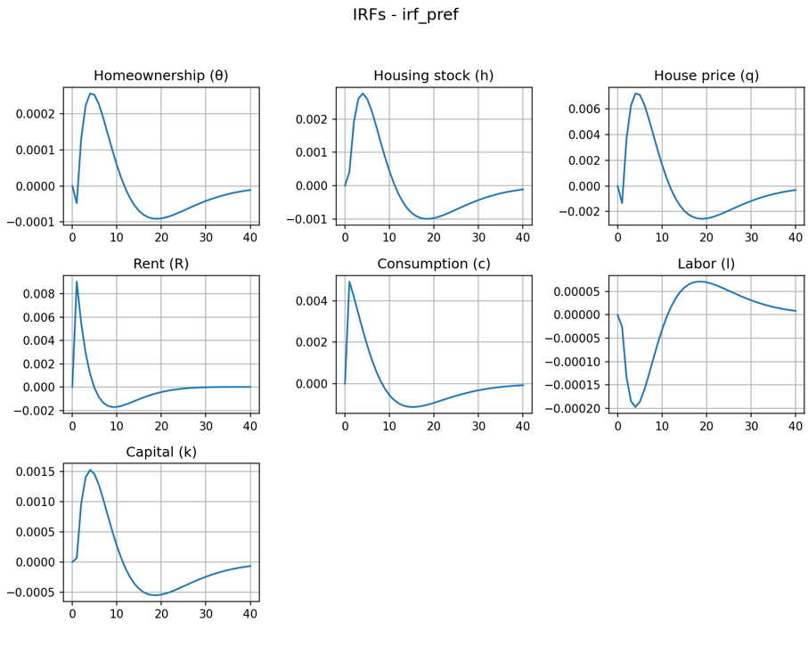
結論
- 嗜好ショック→持ち家率
- 短期
- 嗜好↑(住宅サービスをより好む)
⇒ 当面、賃貸需要>供給 → 影の家賃↑ + 一方で、将来を強く割り引くため住宅価格↓。
⇒ 賃貸の相対魅力↑ → 持ち家率↓
- 嗜好↑(住宅サービスをより好む)
- 中期
- 住宅投資が入り供給↑
⇒ サービス供給が増えて影の家賃↓、住宅価格↓
⇒ 所有の相対魅力↑ → 持ち家率↑
- 住宅投資が入り供給↑
- 長期
- 嗜好↓
⇒ 住宅需要への熱が冷め価格・影の家賃が平常化
⇒ 持ち家率は定常へ回帰
- 嗜好↓
- 短期
今後
- 家計に異質性を導入
- 賃貸市場の導入
- 国内総生産(=総供給)の表示
-
実データによる歴史的分解分析(以下はシミュレーションデータによるもの)

- 価格硬直性、独占的競争市場、金融市場の不完全性を導入
- 政府・中央銀行の導入
- 財政・金融政策の効果検証
- 持ち家率のアドホックなルールを変更
- ロジット関数の利用
\begin{align}
\Delta U_t
&\equiv U_t^{\mathrm{own}} - U_t^{\mathrm{rent}} \\
&\approx s_\xi\bigl(\xi_t - \xi^{ss}\bigr)
\;-\; \kappa_q \bigl(q_t - q^{ss}\bigr)
\;+\; \kappa_R \bigl(R_t - R^{ss}\bigr)
\;-\; \kappa_{\mathrm{adj}} \cdot \bigl(\theta_t - \theta_{t-1}\bigr) \\
\end{align}
\begin{align}
 \theta_t \;=\; \frac{1}{1 + \exp\!\bigl(-\gamma\,\Delta U_t\bigr)}
\qquad (\,0 < \theta_t < 1\,), \quad \gamma>0
\end{align}
- 厚生分析
- 政策介入やショックが家計の効用にどの程度影響するか
- 景気変動の存在は社会的にどれほど「コスト」なのか
- 景気変動を完全に除去した場合、どれだけ厚生が改善するか
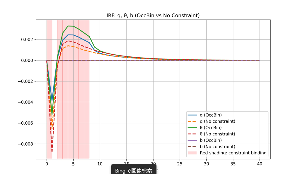
- Occasionally Binding Constraints(時々かかる制約)
- 住宅を担保にした借入制約を実装
- 嗜好ショックのインパルス反応→借入制約は持ち家率を高めるよう機能
- Dynareの活用
- 公式
- マニュアル
- Ubuntu on IBM CloudにOctaveとdynareをインストール + 経済モデルシミュレーション
参考
- 現代マクロ経済学講義―動学的一般均衡モデル入門 加藤 涼
- DSGEモデルによるマクロ実証分析の方法 廣瀬康生
- 動学的一般均衡モデルによる財政政策の分析 江口允崇