(後編 画像オートエンコーダの学習におけるロスの選び方の違い 後編(MIT Places2の場合) 書きました。)
目的
オートエンコーダやVAEなどで画像の再構成のロス(入力画像からの遠さ)を最小化するように学習します。いろいろな実装を見ているとロスの式で二乗誤差ロスを採用しているものとバイナリクロスエントロピロス(logloss?)を採用しているものがありどちらが良いのかいまいちわかりません。また画素単位のロスをそのまま最適化するものとサンプル内で画素毎のロスの平均を取るものがあり、こちらもどちらが良いのかよくわかりません。
最適化の流れから考えれば挙動の違いもなんとなく想像はつくのですがとりあえずベンチマークを取ってしまいます。
注意
- 結果画像として鮮明な顔写真が出てきますがオートエンコーダの出力であり自動生成的なものではありません。「脅威の人工知能実現!」みたいな記事ではありません。
- いろいろと厳密性を欠く実験ではあります。実験の条件は次に述べます。
実験の概要
実験に使用したモデル
前半部分がモデル、後半部分がロスです。特に凝ったことはしていない畳み込み層によるオートエンコーダです。
- 中間の特徴ベクトルサイズは512
- 畳み込み層の活性化関数はReLU
- 線形層の活性化関数はtanh
- デコーダの最終出力の活性化関数はSigmoid
- デコーダの最終出力以外にはバッチノーマライズを使用
- ロスの定義は二乗誤差とバイナリクロスエントロピの2種類を画素毎、サンプル毎、ミニバッチ全体の3通りで計6種類
- オプティマイザはAdam
import tensorflow as tf
import math
from castanea.layers import conv2d, conv2d_transpose, linear, LayerParameter

IMAGE_SUMMARY_MAX_OUTPUTS = 8

LATENT_DIMENTION = 512
WEIGHT_NORMALIZE = False
BATCH_NORMALIZE = True
WITH_BIAS = True
LEARNING_RATE = 1e-4
RECTIFIER = tf.nn.relu
LINEAR_RECTIFIER = tf.tanh
IMAGE_RECTIFIER = tf.sigmoid

def encoder(images):
    ks = 5 # kernel size
    x = images

    p1 = LayerParameter(
        with_bias=WITH_BIAS,
        rectifier=RECTIFIER,
        with_weight_normalize=WEIGHT_NORMALIZE,
        with_batch_normalize=BATCH_NORMALIZE,
        var_device='/gpu:0')
    p2 = LayerParameter(
        with_bias=WITH_BIAS,
        rectifier=LINEAR_RECTIFIER,
        with_weight_normalize=WEIGHT_NORMALIZE,
        with_batch_normalize=BATCH_NORMALIZE,
        var_device='/gpu:0')

    with tf.variable_scope('encoder'):
        x = conv2d(x, ks, ks, 32, parameter=p1)
        x = conv2d(x, ks, ks, 64, strides=[1,2,2,1], parameter=p1)
        x = conv2d(x, ks, ks, 128, strides=[1,2,2,1], parameter=p1)
        x = conv2d(x, ks, ks, 256, strides=[1,2,2,1], parameter=p1)
        x = conv2d(x, ks, ks, 512, strides=[1,2,2,1], parameter=p1)

        x = linear(x, [-1, LATENT_DIMENTION], parameter=p2)

        return x

def decoder(features, core):
    ks = 5 # kernel size

    p1 = LayerParameter(
        with_bias=WITH_BIAS,
        rectifier=RECTIFIER,
        with_weight_normalize=WEIGHT_NORMALIZE,
        with_batch_normalize=BATCH_NORMALIZE,
        var_device='/gpu:0')
    p2 = LayerParameter(
        with_bias=WITH_BIAS,
        rectifier=LINEAR_RECTIFIER,
        with_weight_normalize=WEIGHT_NORMALIZE,
        with_batch_normalize=BATCH_NORMALIZE,
        var_device='/gpu:0')
    p3 = LayerParameter(
        with_bias=WITH_BIAS,
        rectifier=IMAGE_RECTIFIER,
        with_weight_normalize=WEIGHT_NORMALIZE,
        with_batch_normalize=False,
        var_device='/gpu:0')

    with tf.variable_scope('decoder'):
        x = features
        x = linear(x, [-1, core, core, 512], parameter=p2)
        x = conv2d_transpose(x, ks, ks, 256, strides=[1,2,2,1], parameter=p1) # 16
        x = conv2d_transpose(x, ks, ks, 128, strides=[1,2,2,1], parameter=p1) # 32
        x = conv2d_transpose(x, ks, ks, 64, strides=[1,2,2,1], parameter=p1) # 64
        x = conv2d_transpose(x, ks, ks, 32, strides=[1,2,2,1], parameter=p1) # 128
        x = conv2d(x, ks, ks, 3, parameter=p3) # 128

        #tf.summary.image('decoder', x, collections=['image', 'encoder'], max_outputs=IMAGE_SUMMARY_MAX_OUTPUTS )

        return x

def loss_pixel_squared_difference(real_images, generated_images):
    with tf.name_scope('loss'):
        l = tf.squared_difference(real_images, generated_images)
        index_l = l

        l_mean = tf.reduce_mean(l)
        tf.summary.scalar(
            'loss_pixel_squared_difference', l_mean,
            collections=[tf.GraphKeys.SUMMARIES, 'loss', 'scalar'])

        index_l_mean = tf.reduce_mean(index_l) * 1e+7
        tf.summary.scalar(
            'loss_index', index_l_mean, collections=[tf.GraphKeys.SUMMARIES, 'loss', 'scalar'])

        return l

def loss_sample_squared_difference(real_images, generated_images):
    with tf.name_scope('loss'):
        l = tf.squared_difference(real_images, generated_images)
        index_l = l
        l = tf.reduce_mean(l, axis=[0])

        l_mean = tf.reduce_mean(l)
        tf.summary.scalar(
            'loss_sample_squared_difference', l_mean,
            collections=[tf.GraphKeys.SUMMARIES, 'loss', 'scalar'])

        index_l_mean = tf.reduce_mean(index_l) * 1e+7
        tf.summary.scalar(
            'loss_index', index_l_mean, collections=[tf.GraphKeys.SUMMARIES, 'loss', 'scalar'])
        return l

def loss_minibatch_squared_difference(real_images, generated_images):
    with tf.name_scope('loss'):
        l = tf.squared_difference(real_images, generated_images)
        index_l = l
        l = tf.reduce_mean(l)

        l_mean = tf.reduce_mean(l)
        tf.summary.scalar(
            'loss_minibatch_squared_difference', l_mean,
            collections=[tf.GraphKeys.SUMMARIES, 'loss', 'scalar'])

        index_l_mean = tf.reduce_mean(index_l) * 1e+7
        tf.summary.scalar(
            'loss_index', index_l_mean, collections=[tf.GraphKeys.SUMMARIES, 'loss', 'scalar'])
        return l

def loss_pixel_binary_cross_entropy(real_images, generated_images):
    with tf.name_scope('loss'):
        l = - (real_images * tf.log(generated_images + 0.001) +
            (1.0 - real_images) * tf.log(1.0 - generated_images + 0.001))
        index_l = tf.squared_difference(real_images, generated_images)

        l_mean = tf.reduce_mean(l)
        tf.summary.scalar(
            'loss_pixel_binary_cross_entropy', l_mean,
            collections=[tf.GraphKeys.SUMMARIES, 'loss', 'scalar'])

        index_l_mean = tf.reduce_mean(index_l) * 1e+7
        tf.summary.scalar(
            'loss_index', index_l_mean, collections=[tf.GraphKeys.SUMMARIES, 'loss', 'scalar'])
        return l

def loss_sample_binary_cross_entropy(real_images, generated_images):
    with tf.name_scope('loss'):
        l = - (real_images * tf.log(generated_images + 0.001) +
            (1.0 - real_images) * tf.log(1.0 - generated_images + 0.001))
        index_l = tf.squared_difference(real_images, generated_images)
        l = tf.reduce_mean(l, axis=[0])

        l_mean = tf.reduce_mean(l)
        tf.summary.scalar(
            'loss_sample_binary_cross_entropy', l_mean,
            collections=[tf.GraphKeys.SUMMARIES, 'loss', 'scalar'])

        index_l_mean = tf.reduce_mean(index_l) * 1e+7
        tf.summary.scalar(
            'loss_index', index_l_mean, collections=[tf.GraphKeys.SUMMARIES, 'loss', 'scalar'])
        return l

def loss_minibatch_binary_cross_entropy(real_images, generated_images):
    with tf.name_scope('loss'):
        l = - (real_images * tf.log(generated_images + 0.001) +
            (1.0 - real_images) * tf.log(1.0 - generated_images + 0.001))
        index_l = tf.squared_difference(real_images, generated_images)
        l = tf.reduce_mean(l)

        l_mean = tf.reduce_mean(l)
        tf.summary.scalar(
            'loss_minibatch_binary_cross_entropy', l_mean,
            collections=[tf.GraphKeys.SUMMARIES, 'loss', 'scalar'])

        index_l_mean = tf.reduce_mean(index_l) * 1e+7
        tf.summary.scalar(
            'loss_index', index_l_mean, collections=[tf.GraphKeys.SUMMARIES, 'loss', 'scalar'])
        return l

def train(loss, global_step):
    with tf.name_scope('train'):
        opt = tf.train.AdamOptimizer(LEARNING_RATE)
        grads = opt.compute_gradients(loss)
        out = opt.apply_gradients(grads, global_step=global_step)
    return out
実験の条件
- 実験データはCelebA
- 中央領域を切り出し128x128にリサイズして入力画像とする
- データオーグメンテーションとしてランダムで左右反転、輝度変化、コントラスト変化、彩度変化を入れている
- ミニバッチサイズは64
- 各ロスごとに100,000イテレーションの学習を行っている
- 各ロスでの学習において乱数シードの固定はしていない
- 比較のために各ロスでの学習において実験用のロスとは別に二乗誤差基準のロスを出力している
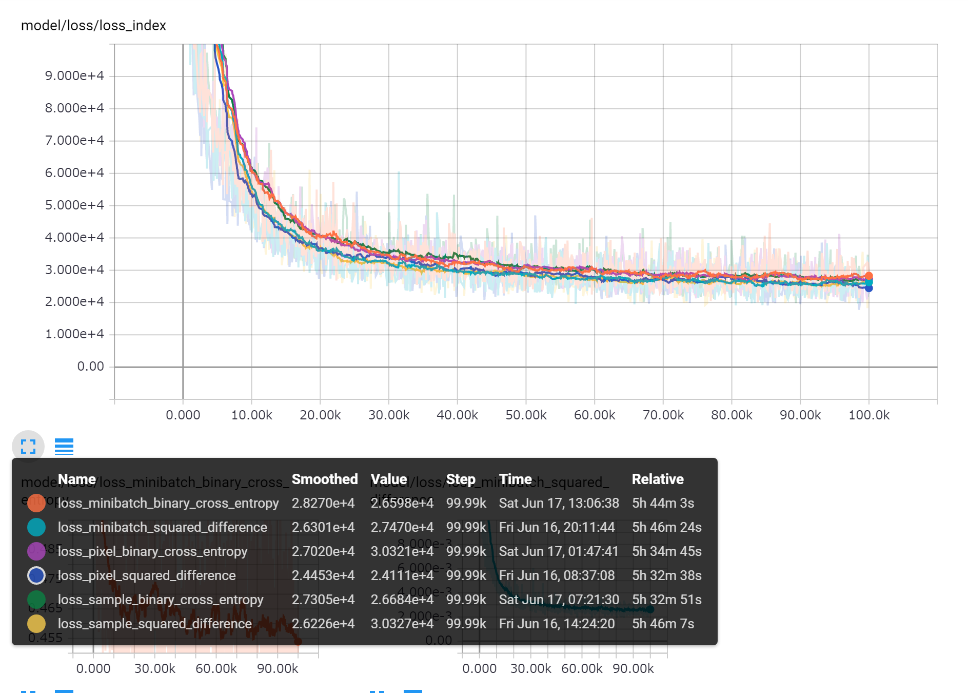
ロスの推移
TensorBoardで学習の推移を表示している。各ロスでの学習時の二乗誤差の推移。チャートを見やすくするために数値に1e+7をかけている。チャートのスムージングは0.95。数値的に若干の差はあるもののほとんど同じ。二乗誤差の下がり方も同じ傾向。
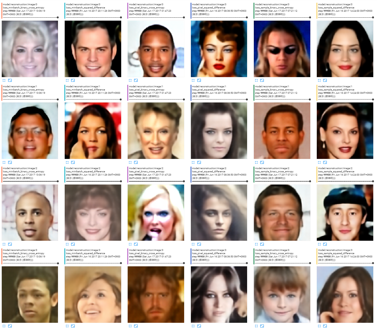
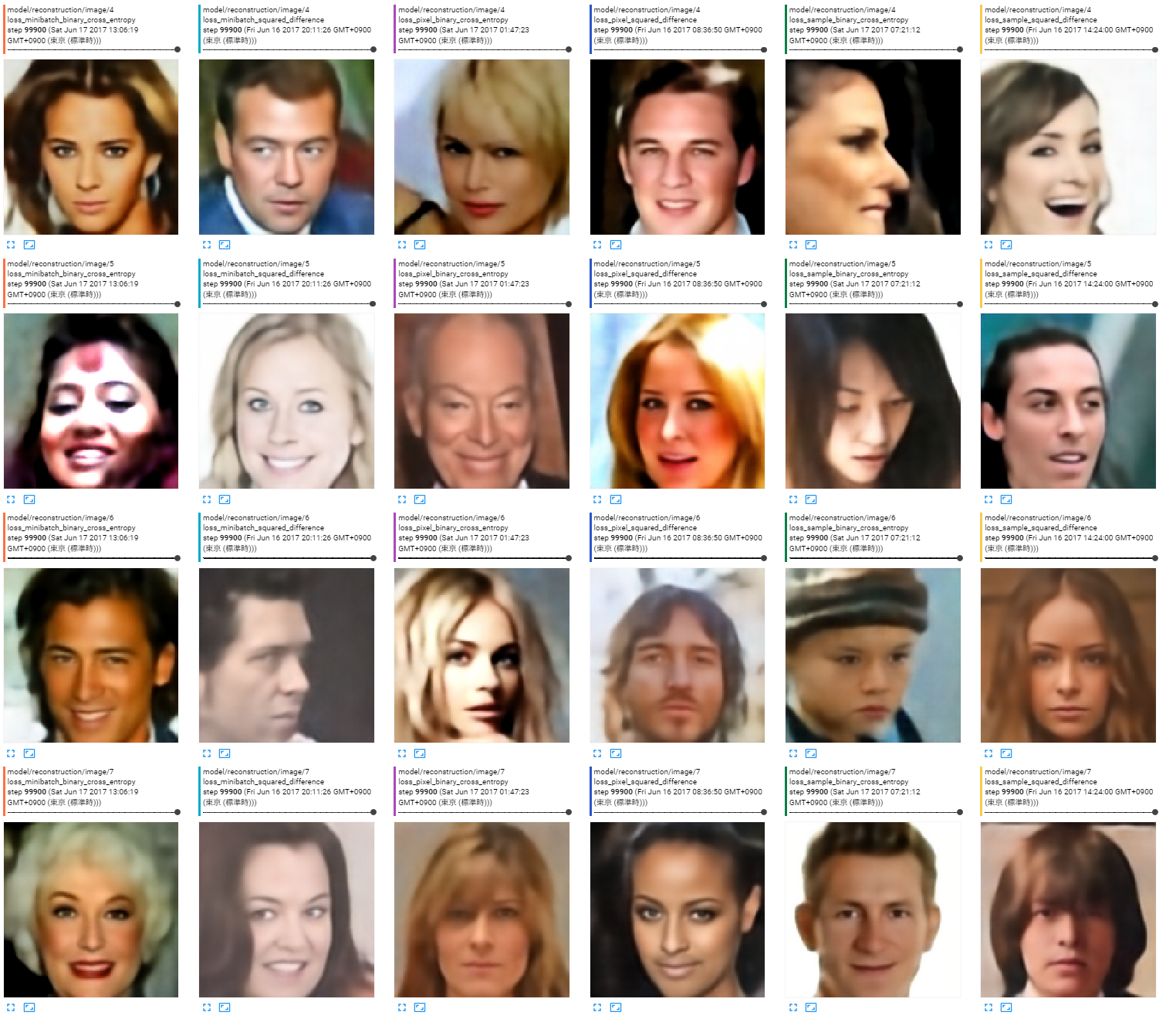
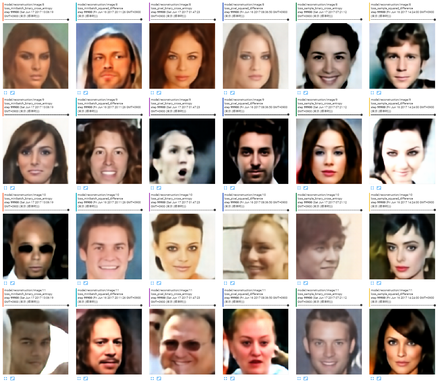
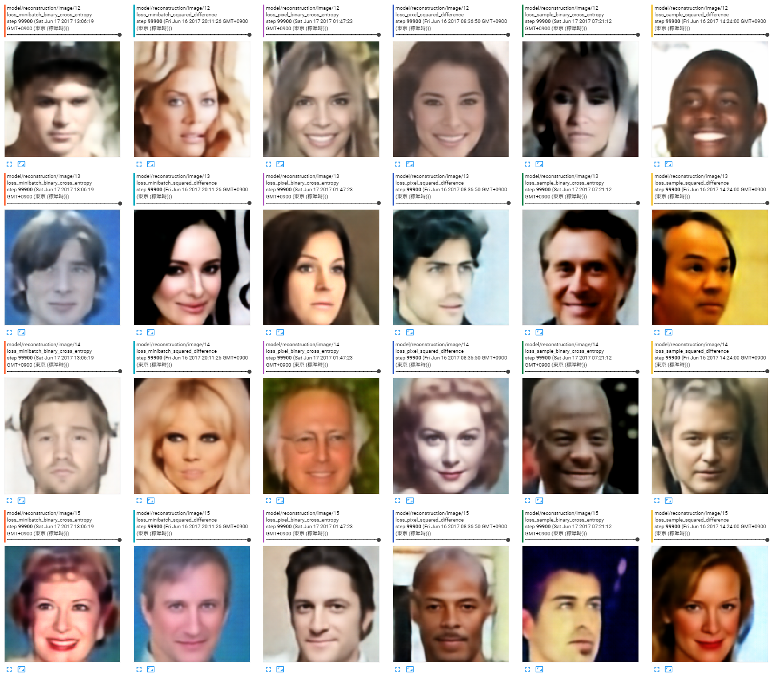
出力画像
どれでもあんまり変わらない。どれでも破綻している画像はある。
ロスの種類は左から以下の順。
- ミニバッチ全体の平均、バイナリクロスエントロピー
- ミニバッチ全体の平均、二乗誤差
- 画素単位、バイナリクロスエントロピー
- 画素単位、二乗誤差
- サンプルごとに平均、バイナリクロスエントロピー
- サンプルごとに平均、二乗誤差
まとめ
どれでもあんまり変わらないんじゃね?という気がします。
ただしCelebAデータセットはクラス内分散がとても小さいので風景データセットや自前のヌード画像データセットを使って分散が大きい場合の傾向も実験したいと思います。
6種類のロスでの実験全部で30時間かかるのが悩みどころ。その間は将棋AIとかができない。