はじめに
この記事ではSTDCによる遺伝的プログラミングを用いた為替市場のトレンド反転点の予測についてまとめました。
STDCや遺伝的プログラミングについて、「?」という方も問題なく読み進めますのでご安心ください。
元論文は以下になります。
注意
これは個人で作成したコードです。誤りなどの可能性がありますが、ご容赦ください。
1. なぜ実装したか
私は機械学習・深層学習を用いた個人開発をする際に、「自身を含めたユーザが活用を実感できる」をテーマに開発を行っています。
その一環として、以前より株式や為替市場の予測モデル関する論文を読んだり実装をしてきました。正確な予測モデルが実装できれば、EAなどに組み込むことでユーザの金銭的利益につながると考えます。スタンダードなモデルとしては LSTM などの時系列モデルや LightGBM 等の勾配ブースティング木などが使用されることが多いです。これらのモデルを利用した論文では、実際に高い精度を叩き出しているものもあります。
しかし、これらのStock Market、Forex系統の論文で以下のように異常に高い予測精度を示しているモデルには注意しなければなりません。
lag-model という現象が発生している危険性があるためです。
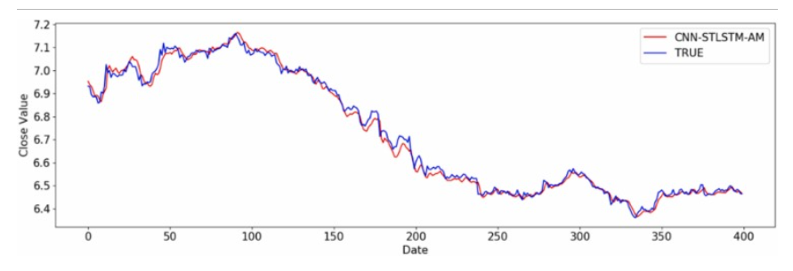
(引用:A CNN-STLSTM-AM model for forecasting USD/RMB exchange rate)
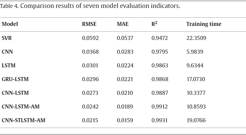
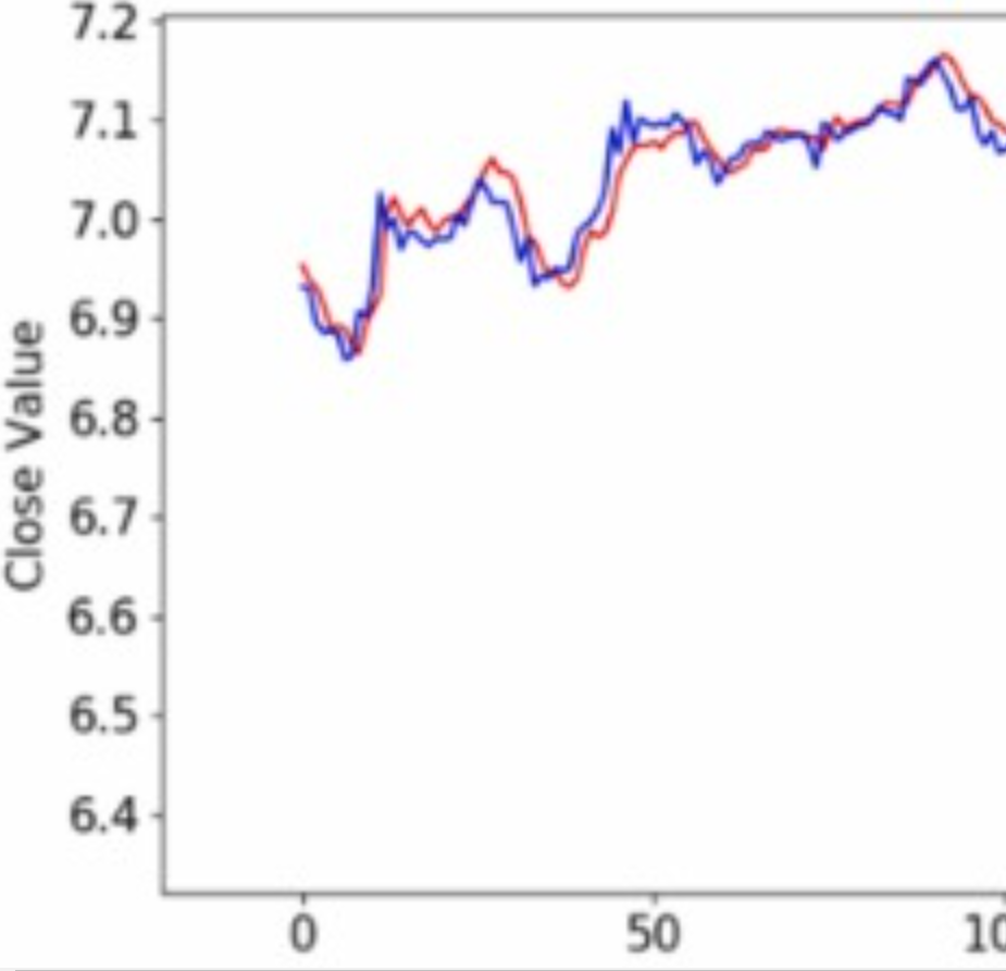
時系列のグラフと決定係数の数値を見るに、モデルの予測精度が異常に高いことが見て取れます。
しかし、グラフを拡大して見てみると実測値と予測値が時系列方向にズレていることが分かります。
これは一般に lag-model (遅延モデル) と呼ばれ、予測値が特定ステップ数前のデータを強く参照してしまい、実測値の推移が予測値の推移を追いかけるようなモデルとなってしまう現象です。
そのため、リアルタイムで動作させると現在の時系列データから現在の価格を出力するといった意味不明なモデルが出来上がってしまいます。
他にもこの現象の特徴として、RMSE や 決定係数 等の評価指標が異常に高い傾向があると確認されています。
このような株式・為替予測モデルにおいて、多くのモデルがlag-modelと化してしまい、正常な予測が出来ていないのが現状です。
正確な予測モデルを作成するためにはlag-modelを発生させない、つまりは価格の予測を行わずに利益を発生させる予測システムを実装する必要があります。
そこで、為替市場における予測に関して「STDCによる遺伝的プログラミングを用いた為替市場のトレンド反転点の予測」という有用なアプローチを取っている論文を発見したので、実際に実装して制度を確認してみました。
2. STDCとは
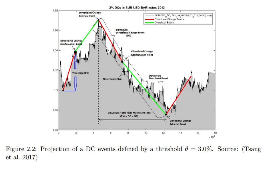
STDCとは Single Threshold Directional Change の略称です。この手法を用いると、株式や為替の時系列データを上昇・下降トレンドに区分することが出来ます。
(引用:ESTIMATING DIRECTIONAL CHANGES TREND
REVERSAL IN FOREX USING MACHINE LEARNING)
STDCでは DC(Directional Change)イベント と OS(OverShoot)イベント の2つに区分されます。
ユーザが任意に設定した Threshold(閾値) を基に高値と底値から一定の変動があった場合トレンドが転換していると定義しています。
トレンドが転換した際にDCイベントが発生します。DCイベントの発生後、現在の価格が高値や底値を更新すると、その期間がOSイベントとなります。
基本的にDCイベントとOSイベントはセットで考えて構いません。しかし、トレンド転換後、経済指標等の発表が重なり運悪く大きな価格変動があった場合はOSイベントを経由せず、DCイベントが発生することがあります。
このSTDCを用いて時系列データから、新たにDCイベントとOSイベントから構築された新たなデータセットを作成し、それを学習モデルに活用しています。
以下は時系列データをDC-OSイベントが発生した時系列データをデータセットとして出力するコードになります。(以下はグラフ描画用のコードです。データセット用のコードは別途紹介します。)
import pandas as pd
import numpy as np
import matplotlib.pyplot as plt

class DCEventDetector:
    def __init__(self, dataframe, delta):
        self.eventsDC = []
        self.eventsOS = []
        self.delta = delta
        self.indexDC = [0, 0]
        self.indexOS = [0, 0]
        self.dataframe = dataframe

    def generateDC(self):
        countDC = 0
        countOS = 0
        delta = self.delta
        df = self.dataframe

        for index in range(len(df)):
            price = df.iloc[index]
            if (index == 0): #初期設定
                type = "Upturn"
                high = df.iloc[index]
                low = df.iloc[index]
                isExistOS = False

            else:
                if (type == "Upturn"):
                    if (price <= (high * (1 - delta))): #上昇トレンドから下降トレンドに転換
                        if (self.indexOS[0] >= self.indexOS[1]):
                            isExistOS = False
                        if (isExistOS is False):
                            if (countDC == 0):
                                countDC += 1
                                self.eventsDC.append((0, df.iloc[0], index, price, "DC Upturn", countDC))
                                #print(f"Upturn DCC with not OS at 0, DC count {countDC}, indexDC[0] {self.indexDC[0]}, indexDC[1] {index}, indexOS[0] {self.indexOS[0]}, indexOS[1] {self.indexOS[1]}")


                            else:
                                countDC += 1
                                self.eventsDC.append((self.indexDC[0], df.iloc[self.indexDC[0]], index, price, "DC Upturn", countDC))
                                self.indexDC[0] = self.indexDC[1] + 1
                                #print(f"Upturn DCC with not OS, DC count {countDC}, indexDC[0] {self.indexDC[0]}, indexDC[1] {index}, indexOS[0] {self.indexOS[0]}, indexOS[1] {self.indexOS[1]}")
                        else:
                            countDC += 1
                            countOS = countDC - 1
                            self.eventsDC.append((self.indexDC[0], df.iloc[self.indexDC[0]], index, price, "DC Upturn", countDC))
                            self.eventsOS.append((self.indexOS[0], df.iloc[self.indexOS[0]], self.indexOS[1] , df.iloc[self.indexOS[1]] , "OS Upturn", countOS))
                            #print(f"Upturn DCC with OS , DC count {countDC}, indexDC[0] {self.indexDC[0]}, indexDC[1] {index}, indexOS[0] {self.indexOS[0]}, indexOS[1] {self.indexOS[1]}")

                        self.indexDC[1] = index
                        self.indexOS[0] = index + 1
                        low = price
                        isExistOS = False
                        type = "Downturn"
                        #print(f"Change Index indexDC[0] {self.indexDC[0]}, indexDC[1] {self.indexDC[1]}, indexOS[0] {self.indexOS[0]}, indexOS[1] {self.indexOS[1]}")
                        continue

                    elif (high < price):
                        high = price
                        self.indexDC[0] = index
                        self.indexOS[1] = index - 1
                        isExistOS = True
                        #print(f"Upturn OS is valid, DC count {countDC}, indexDC[0] {self.indexDC[0]}, indexDC[1] {self.indexDC[1]}, indexOS[0] {self.indexOS[0]}, indexOS[1] {self.indexOS[1]}")

                    else:
                        #print("continue")
                        continue


                elif (type == "Downturn"):
                    if (price >= (low * (1 + delta))): #下降トレンドから上昇トレンドに転換
                        if (self.indexOS[0] >= self.indexOS[1]):
                            isExistOS = False
                        if (isExistOS is False):
                            #print(f"Downturn DCC with not OS, DC count {countDC}, indexDC[0] {self.indexDC[0]}, indexDC[1] {index}, indexOS[0] {self.indexOS[0]}, indexOS[1] {self.indexOS[1]}")
                            countDC += 1
                            self.eventsDC.append((self.indexDC[0], df.iloc[self.indexDC[0]], index, price, "DC Downturn", countDC))
                            self.indexDC[0] = self.indexDC[1] + 1

                        else:
                            countDC += 1
                            countOS = countDC -1
                            self.eventsDC.append((self.indexDC[0], df.iloc[self.indexDC[0]], index, price, "DC Downturn", countDC))
                            self.eventsOS.append((self.indexOS[0], df.iloc[self.indexOS[0]], self.indexOS[1] , df.iloc[self.indexOS[1]] , "OS Downturn", countOS))
                            #print(f"Downturn DCC with OS, DC count {countDC}, indexDC[0] {self.indexDC[0]}, indexDC[1] {index}, indexOS[0] {self.indexOS[0]}, indexOS[1] {self.indexOS[1]}")

                        self.indexDC[1] = index
                        self.indexOS[0] = index + 1
                        high = price
                        isExistOS = False
                        type = "Upturn"
                        #print(f"Change Index indexDC[0] {self.indexDC[0]}, indexDC[1] {index}, indexOS[0] {self.indexOS[0]}, indexOS[1] {self.indexOS[1]}")
                        continue

                    elif (low > price):
                        low = price
                        self.indexDC[0] = index
                        self.indexOS[1] = index - 1
                        isExistOS = True
                        #print(f"Downturn OS is valid, DC count {countDC}, indexDC[0] {self.indexDC[0]}, indexDC[1] {self.indexDC[1]}, indexOS[0] {self.indexOS[0]}, indexOS[1] {self.indexOS[1]}")

                    else:
                        #print("continue")
                        continue

        df_DC = pd.DataFrame(self.eventsDC, columns=["DC_Start_Index", "Price_DC_Start", "DC_End_Index", "Price_DC_End", "DC_Type", "Number"])
        df_OS = pd.DataFrame(self.eventsOS, columns=["OS_Start_Index", "Price_OS_Start", "OS_End_Index", "Price_OS_End", "OS_Type", "Number"])

        #最後のDCイベントにはOSイベントが続かないため削除
        df_DC = df_DC.iloc[:-1]
        df_OS = df_OS.iloc[1:]

        return df_DC, df_OS

phyisical_time_df = pd.read_csv('./USDJPY_10 Mins_Ask_2003.05.04_2024.03.29.csv')
price_df = phyisical_time_df["Close"]
dc_generator = DCEventDetector(price_df, 0.1)
df_dc, df_os = dc_generator.generateDC()

def plot_events_with_lines(price_df, df_dc, df_os):

    plt.figure(figsize=(30, 10))
    plt.plot(price_df)
    plt.scatter(df_dc["DC_Start_Index"], df_dc["Price_DC_Start"], color="orange", label='DC Start')
    plt.scatter(df_dc["DC_End_Index"], df_dc["Price_DC_End"], color="red", label='DC End')
    plt.scatter(df_os["OS_Start_Index"], df_os["Price_OS_Start"], color="cyan", label='OS Start')
    plt.scatter(df_os["OS_End_Index"], df_os["Price_OS_End"], color="blue", label='OS End')


    plt.legend()
    plt.show()

plot_events_with_lines(price_df, df_dc, df_os)
※余談ですが、DCイベントの平均の長さとOSイベントの平均の長さの間で、以下の関係式が成り立つことが分かっています。
OS ≃2 × DC
実際にDCイベントの長さとOSイベントの長さの比をヒストグラムでまとめてみました。(閾値は多くの比率を比較するため0.005に設定しました。)
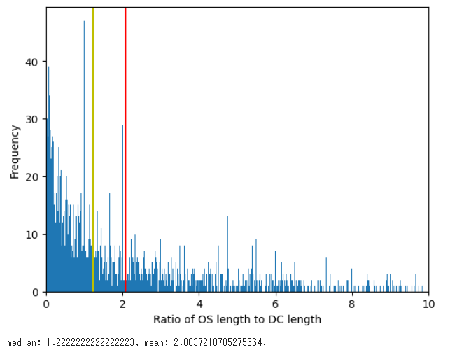
※全データから 第三四分位数+1.5×IQR を基準に外れ値を取り除いています。
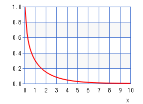
また、比率の分布は χ二乗分布(以下は自由度1.5、増分は0.1) で近似できると考えられるので、この法則を有用に使えば機械学習・深層学習を利用せず統計的に自動売買が行える可能性があります。
3. 遺伝的プログラミングとは
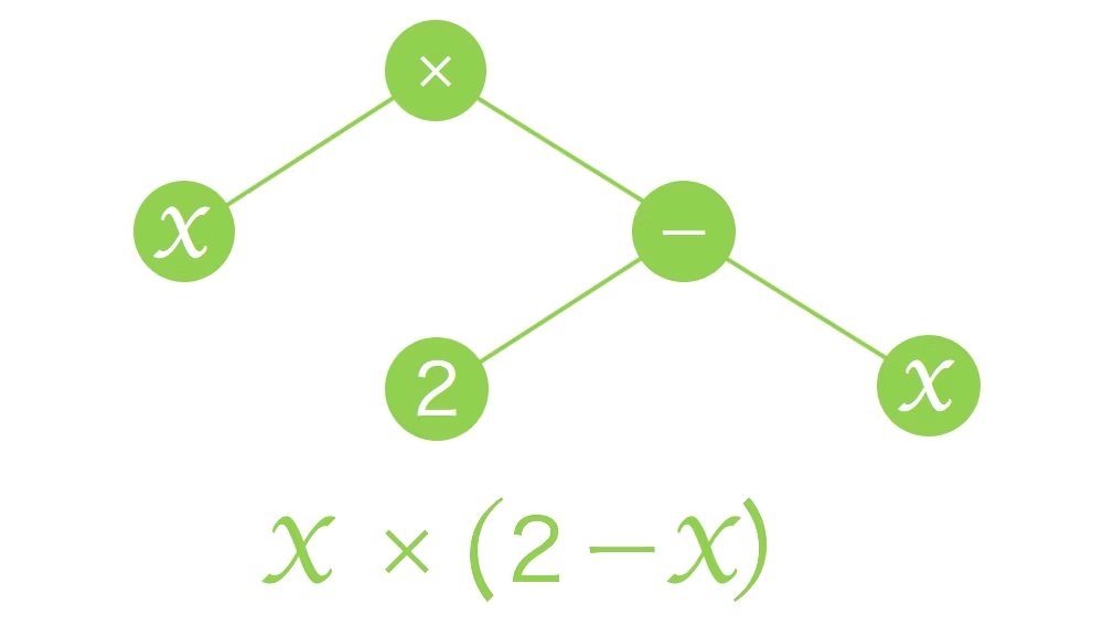
遺伝的プログラミングとは、簡単に言ってしまえば 変数間の関係式を逐次的に生成するアルゴリズムです。構造には主に木構造が用いられています。
名前にもある通り、生物の遺伝的性質 をアルゴリズムに応用しています。
以下は、遺伝的プログラミングの概要です。
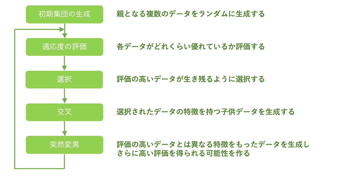
(引用:遺伝的アルゴリズムと遺伝的プログラミングを自力で実装して理解する)
初期集団を生成した後、3つの処理(選択、交叉、突然変異)により新たな関係式を生成し新たな集団とします。適応度が最適な値になるか、世代交代の回数が規定値にまで達するまで、これを繰り返します。
次に遺伝的プログラミングの重要なキーワードについて解説します。
| キーワード | 意味 |
|---|---|
| 初期化 | 比較元となる関係式を生成する方法論。grow 法、full 法、half and half 法などがある。 |
| 適応度 | 生成した関係式を評価する関数。機械学習や深層学習における損失関数と同じ位置付け。MSE や RMSE、決定係数 を使用することが多い。 |
| 選択 | 生成した関係式から優秀なものを抽出する方法論。 ルーレット選択 や トーナメント選択 など様々な選択方法がある。 |
| 交叉 | 生成した関係式から新たな関係式を生成する方法。2つの関係式を示す木構造からランダムにサブツリーを選択し、それを新たな関係式とする |
| 突然変異 | 生成した関係式の構造をランダムに変更する方法論。関係式の進化の早期収束を防止できる。サブツリー突然変異 や ホイスト突然変異、ポイント突然変異 などがある。 |
ここでは、説明変数の分布から目的変数を表現する最適なモデルを構築する、深層学習でいうところの 回帰モデル を生成しているという認識で構いません。
わざわざ遺伝的プログラミングという手法を取っているのは以下の理由があります。
- OSイベントの長さはDCイベントの長さの平均2倍になる という2値間の関係性が判明していたため、比較的簡易な関係式で表現できると考えられた。
- 為替取引に使用する以上、リアルタイム性が求められるため、LSTMや等の時系列モデルより高速である必要がある。
各方法論や詳細な処理について知りたい方は、以下のサイトや記事が参考になるのでぜひご覧になってください。
4. モデル構造
モデル構造の概要は以下の通りになります。
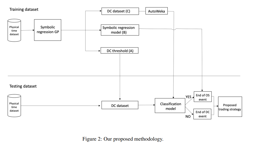
処理の流れは以下になります。
- 任意の閾値範囲から一つ閾値を選択し、各閾値ごとで訓練データからDC-OSデータセットを作成する。
- 遺伝的プログラミングを用いて、各DC-OSデータセットごとの最適な関係式を生成する。
- 各閾値ごとの最適な関係式を比較し、最も適合度が高い(閾値、DC-OSデータセット、関係式)を探索する。
- 3.で獲得したDC-OSデータセットを用いて、DCイベントがOSイベントを持つかどうかを判別する2値分類モデルを作成する。
- 1.~ 4.で得た(閾値、関係式、判別モデル)を利用して、まず評価データをDC-OSデータセットを作成する。
- 判別モデルでDCイベントがOSイベントを持つと判断したときのDCイベントの長さを関係式に入力しOSイベントの長さを予測、評価する。
5. 学習
5.1. データセットの作成
2. STDCとは の項目でご説明したコードですが、これは描画用のコードです。実際にデータセットとして使用するには適しておりません。
理由として、このコードだとDCイベントには必ずOSイベントが付随してしまい、判別モデルに入力できなくなるためです。以下のコードでは、DCイベントの急激な変動を1ステップだけではなく、3ステップ程度のマージンを確保することでモデルに遊びを予備しています。
class Event:
    def __init__(self, start, start_price, end, end_price, event_type, percentage_displacement=0):
        self.start = start
        self.start_price = start_price
        self.end = end
        self.end_price = end_price
        self.event_type = event_type
        self.overshoot = None
        self.percentage_displacement = percentage_displacement

class Type:
    Upturn = "Upturn"
    Downturn = "Downturn"
    UpwardOvershoot = "UpwardOvershoot"
    DownwardOvershoot = "DownwardOvershoot"

def generate_events(price_df, delta):
    events = []
    event = Type.Upturn

    last = Event(-1, 0, -1, 0, Type.Upturn)
    events.append(last)

    p_high = 0
    p_low = 0

    index_dc = [-1, -1]  # DC event indexes
    index_os = [-1, -1]  # OS event indexes
    index = 1

    for index, price in enumerate(price_df):
        if index == 0:
            p_high = price
            p_low = price

            index_dc = [index] * 2
            index_os = [index] * 2
        elif event == Type.Upturn:
            if price <= (p_high * (1 - delta)):
                last.overshoot = detect(price_df, Type.UpwardOvershoot, index_dc, index_os)


                adjust(last.overshoot if last.overshoot else last, index_dc, index_os)


                event = Type.Downturn
                p_low = price

                index_dc[1] = index
                index_os[0] = index + 1

                last = Event(index_dc[0], price_df.iloc[index_dc[0]], index_dc[1], price_df.iloc[index_dc[1]], Type.Downturn)
                events.append(last)

            elif p_high < price:
                p_high = price

                index_dc[0] = index
                index_os[1] = index - 1
        else:
            if price >= (p_low * (1 + delta)):
                last.overshoot = detect(price_df, Type.DownwardOvershoot, index_dc, index_os)


                adjust(last.overshoot if last.overshoot else last, index_dc, index_os)

                event = Type.Upturn
                p_high = price

                index_dc[1] = index
                index_os[0] = index + 1

                last = Event(index_dc[0], price_df.iloc[index_dc[0]], index_dc[1], price_df.iloc[index_dc[1]], Type.Upturn)
                events.append(last)

            elif p_low > price:
                p_low = price

                index_dc[0] = index
                index_os[1] = index - 1

    return events

def detect(price_df, event_type, index_dc, index_os):
    if index_os[0] < index_os[1] and index_os[0] < index_dc[0]:
        return Event(index_os[0], price_df.iloc[index_os[0]], index_os[1], price_df.iloc[index_os[1]], event_type)
    return None

def adjust(last, index_dc, index_os):
    if index_dc[0] == last.start:
        index_dc[0] = last.end + 1
    elif index_dc[0] > (last.end + 1):
        index_dc[0] = (last.end + 1)

def output_dataframe_dc_os(price_df, threshold):

    events = generate_events(price_df, threshold)

    data = []

    for event in events:
        add_data = {
            "startIndexDC": int(event.start),
            "startPriceDC": event.start_price,
            "endIndexDC": int(event.end),
            "endPriceDC": event.end_price,
            "DC_type": event.event_type,
            "startIndexOS": int(event.overshoot.start) if event.overshoot else None,
            "startPriceOS": event.overshoot.start_price if event.overshoot else None,
            "endIndexOS": int(event.overshoot.end) if event.overshoot else None,
            "endPriceOS": event.overshoot.end_price if event.overshoot else None,
            "OS_type": event.overshoot.event_type if event.overshoot else None
        }
        data.append(add_data)

    df_dc_os = pd.DataFrame(data)

    df_dc_os = df_dc_os.iloc[1:]

    return df_dc_os

def output_datafraome_classification(price_df, threshold):

    df_dc_os = output_dataframe_dc_os(price_df, threshold)

    df_classification = df_dc_os.copy()
    df_classification["PreviousOS"] = df_classification["OS_type"].shift(1)
    df_classification["PreviousOS"] = df_classification["PreviousOS"].apply(lambda x: 1 if x !=None else 0)
    df_classification["TimeDifference"] = (df_classification["endIndexDC"] - df_classification["startIndexDC"]) * 10
    df_classification["CurrentTmv"] = ((df_classification["endPriceDC"] - df_classification["startPriceDC"]) / df_classification["startPriceDC"]) / threshold
    df_classification["PreviousDCPrice"] = df_classification["endPriceDC"].shift(1)
    df_classification["Sigma"] = df_classification.apply(lambda x: (x["CurrentTmv"] * threshold) / x["TimeDifference"] if x["TimeDifference"] != 0 else -1, axis=1)
    df_classification["FlashEvent"] = df_classification.apply(lambda x: 1 if (x["endIndexDC"] == x["startIndexDC"]) else 0, axis=1)
    df_classification["IsOS"] = df_classification.apply(lambda x: 1 if x["OS_type"] != None else 0, axis=1)

    df_classification = df_classification.drop(columns=["startIndexDC", "startPriceDC", "endIndexDC", "endPriceDC", "DC_type", "startIndexOS", "startPriceOS", "endIndexOS", "endPriceOS", "OS_type"])

    df_classification = df_classification[1:]

    return df_classification

phyisical_time_df = pd.read_csv('./USDJPY_10 Mins_Ask_2003.05.04_2024.03.29.csv')
price_df = phyisical_time_df["Close"]
threshold = 0.0025
df_classification = output_datafraome_classification(price_df, threshold)
作成したデータセットは以下のようになります。最初の行を除外しているのは、最初に判別したOSイベントにはDCインベントが付随していないためです。
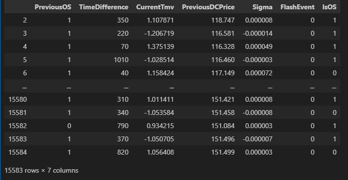
各変数の説明は以下の通りになります。
| 変数名 | 意味 |
|---|---|
| PreviousOS | DCイベントの前にOSイベントがあったかどうか。 |
| TimeDifference | DCイベントの長さ。 |
| CurrentTmv | (DCイベントの終了地点の価格-開始地点の価格)/閾値 |
| PreviousDCPrice | 前のDCイベントの終了地点の価格 |
| Sigma | CurrentTmv × 閾値 / TimeDifference |
| FlashEvent | 価格の急変動後に発生したDCイベントがどうか。 |
| IsOS | OSイベントを持つかどうか。目的変数。 |
5.2. 遺伝的プログラミングの学習
遺伝的プログラミングの実装について、gplearn というpythonライブラリを使用しました。以下のリンクから使用方法などを確認できますので、よろしければ参考にしてください。
sklearnを基にしたライブラリであり、数行のコードで学習評価ができることが大きな特徴です。
gplearnを利用する方法は1行で済みます。
pip install gplearn
以下は遺伝的プログラミングを学習させるコードになります。
from gplearn.genetic import SymbolicRegressor

def gpTuning(X, y, population_size, generations,
             tournament_size, stopping_criteria, const_range, init_Depth, init_method,
             function_set, metric, parsimony_coefficient, p_crossover, p_subtree_mutation,
             p_hoist_mutation, p_point_mutation, p_point_replace, n_jobs, verbose, random_state):

    model = SymbolicRegressor(population_size=population_size, generations=generations, stopping_criteria=stopping_criteria, const_range=const_range,
                                         init_depth=init_Depth, init_method=init_method, function_set=function_set, metric=metric, parsimony_coefficient=parsimony_coefficient,
                                         p_crossover=p_crossover, p_subtree_mutation=p_subtree_mutation, p_hoist_mutation=p_hoist_mutation, p_point_mutation=p_point_mutation,
                                         p_point_replace=p_point_replace, tournament_size=tournament_size, n_jobs=n_jobs, verbose=verbose, random_state=random_state)

    optimized_model = model.fit(X, y)


    return optimized_model

def outputBestFitnessAndModel(optimized_model_list):
    tmp_fitness = np.inf
    for model in optimized_model_list:
        fitness = model._best_fitness
        if (fitness < tmp_fitness):
            best_fitness = fitness
            best_model = model

    return best_fitness, best_model


def outputBestThresholdAndModel(price_df, min_threshold, max_threshold, population_size, generations, tournament_size,
                              stopping_criteria, const_range, init_Depth, init_method, function_set, metric,
                              parsimony_coefficient, p_crossover, p_subtree_mutation, p_hoist_mutation,
                              p_point_mutation, p_point_replace, n_jobs, verbose, random_state):

    optimized_model_list = []
    for threshold in np.arange(min_threshold, max_threshold, 0.0005):
        df = price_df.copy()
        df_dc_os = output_dataframe_dc_os(price_df, threshold)

        X = (df_dc_os["endIndexDC"] - df_dc_os["startIndexDC"]).values.reshape(-1, 1)
        y = (df_dc_os["startIndexOS"] - df_dc_os["endIndexOS"]).values.reshape(-1, 1)


        optimized_model = gpTuning(X, y, population_size=population_size, generations=generations, tournament_size=tournament_size, stopping_criteria=stopping_criteria, const_range=const_range,
                                  init_Depth=init_Depth, init_method=init_method, function_set=function_set, metric=metric, parsimony_coefficient=parsimony_coefficient,
                                  p_crossover=p_crossover, p_subtree_mutation=p_subtree_mutation, p_hoist_mutation=p_hoist_mutation, p_point_mutation=p_point_mutation,
                                  p_point_replace=p_point_replace, n_jobs=n_jobs, verbose=verbose, random_state=random_state)

        optimized_model_list.append(optimized_model)

    return optimized_model_list

optimized_model_list = outputBestThresholdAndModel(price_df, min_threshold=0.005, max_threshold=0.01, population_size=1000, generations=100, tournament_size=20,
                            stopping_criteria=3, const_range=(0, 10), init_Depth=(3, 9), init_method='half and half',
                            function_set=('add', 'sub', 'mul', 'div', 'log', 'sin', 'cos'),
                            metric='rmse', parsimony_coefficient='auto', p_crossover=0.96, p_subtree_mutation=0.01, p_hoist_mutation=0.01,
                            p_point_mutation=0.01, p_point_replace=0.01, n_jobs=4, verbose=1, random_state=1234)
以下は学習結果になります。
---- ------------------------- ------------------------------------------ ----------
Gen Length Fitness Length Fitness OOB Fitness Time Left
0 59.31 1.55136e+12 21 179.079 N/A 1.45m
1 6.71 19227.2 6 181.223 N/A 21.30s
2 2.14 2674.54 3 187.444 N/A 19.49s
3 1.13 194.211 1 189.727 N/A 19.70s
4 1.06 189.973 3 187.373 N/A 19.39s
5 1.07 236.665 3 188.777 N/A 19.19s
6 1.14 197.62 1 189.727 N/A 18.85s
7 1.03 189.919 1 189.727 N/A 20.36s
8 1.05 193.569 1 189.727 N/A 39.66s
9 1.07 190.075 1 189.727 N/A 19.89s
10 1.07 236.637 12 186.774 N/A 19.30s
11 1.02 190.034 3 187.439 N/A 17.78s
12 1.04 236.662 1 189.727 N/A 17.73s
13 1.06 190.328 1 189.727 N/A 18.80s
14 1.07 190.018 3 187.395 N/A 18.77s
15 1.15 236.482 3 187.195 N/A 18.40s
16 1.05 190.153 1 189.727 N/A 19.26s
17 1.08 190.453 3 188.895 N/A 17.78s
18 1.02 189.877 3 186.849 N/A 17.70s
19 1.06 190.238 7 187.994 N/A 22.40s
20 1.08 283.997 1 189.727 N/A 17.35s
21 1.09 196.382 1 189.727 N/A 15.91s
22 1.07 237.168 1 189.727 N/A 16.65s
23 1.04 190.102 3 188.97 N/A 16.69s
24 1.04 190.115 3 189.202 N/A 16.47s
25 1.04 190.556 1 189.727 N/A 17.36s
26 1.02 189.896 1 189.727 N/A 16.04s
27 1.07 190.655 3 187.246 N/A 15.60s
28 1.05 236.804 3 187.61 N/A 15.73s
29 1.05 190.948 1 189.727 N/A 16.26s
30 1.08 237.227 1 189.727 N/A 15.25s
31 1.05 190.234 1 189.727 N/A 21.27s
32 1.05 190.497 1 189.727 N/A 14.73s
33 1.01 189.828 3 188.914 N/A 15.30s
34 1.02 189.858 3 187.599 N/A 14.19s
35 1.03 236.748 1 189.727 N/A 13.99s
36 1.11 237.705 1 189.727 N/A 15.01s
37 1.18 234.43 1 189.727 N/A 14.57s
38 1.03 190 1 189.727 N/A 14.28s
39 1.11 190.201 6 188.352 N/A 13.02s
40 1.02 189.9 1 189.727 N/A 12.93s
41 1.03 190 1 189.727 N/A 13.70s
42 1.06 189.916 1 189.727 N/A 12.34s
43 1.07 190.025 1 189.727 N/A 12.37s
44 1.05 189.891 3 187.414 N/A 18.10s
45 1.05 189.925 1 189.727 N/A 12.68s
46 1.06 190.385 1 189.727 N/A 11.62s
47 1.03 190.632 1 189.727 N/A 12.16s
48 1.12 190.055 1 189.727 N/A 11.13s
49 1.05 51967.1 6 188.386 N/A 11.79s
50 1.02 190.224 3 189.362 N/A 12.30s
51 1.13 250.066 1 189.727 N/A 11.32s
52 1.02 190.3 3 188.832 N/A 11.00s
53 1.04 236.956 1 189.727 N/A 11.44s
54 1.05 193.413 3 188.912 N/A 10.42s
55 1.06 190.753 1 189.727 N/A 9.75s
56 1.06 190.99 3 189.244 N/A 10.13s
57 1.07 189.966 1 189.727 N/A 11.02s
58 1.03 237.271 1 189.727 N/A 9.69s
59 1.07 190.243 1 189.727 N/A 9.43s
60 1.05 189.942 1 189.727 N/A 9.09s
61 1.12 194.171 1 189.727 N/A 13.64s
62 1.07 555.542 1 189.727 N/A 9.27s
63 1.11 190.625 1 189.727 N/A 8.95s
64 1.12 289.839 1 189.727 N/A 8.27s
65 1.03 189.889 1 189.727 N/A 8.48s
66 1.03 190.097 3 189.173 N/A 7.77s
67 1.06 336.906 3 189.108 N/A 7.75s
68 1.11 512.643 3 188.718 N/A 7.66s
69 1.01 189.865 3 189.482 N/A 7.59s
70 1.07 236.952 1 189.727 N/A 6.78s
71 1.04 190.704 6 186.922 N/A 6.99s
72 1.08 190.026 1 189.727 N/A 6.69s
73 1.11 189.941 1 189.727 N/A 6.51s
74 1.07 217.633 1 189.727 N/A 6.24s
75 1.06 190.184 1 189.727 N/A 5.60s
76 1.05 189.946 1 189.727 N/A 5.38s
77 1.05 237.285 1 189.727 N/A 5.46s
78 1.11 190.062 1 189.727 N/A 5.22s
79 1.11 190.817 1 189.727 N/A 5.06s
80 1.03 189.968 1 189.727 N/A 4.67s
81 1.03 79277.8 1 189.727 N/A 7.07s
82 1.10 283.71 7 188.409 N/A 4.25s
83 1.10 241.096 12 189.267 N/A 3.97s
84 1.04 236.941 3 187.725 N/A 3.53s
85 1.02 190.578 1 189.727 N/A 3.30s
86 1.02 189.964 1 189.727 N/A 3.23s
87 1.05 190.428 1 189.727 N/A 3.00s
88 1.08 190.184 1 189.727 N/A 2.75s
89 1.05 236.649 1 189.727 N/A 2.67s
90 1.04 189.936 7 189.352 N/A 2.39s
91 1.07 190.196 1 189.727 N/A 1.97s
92 1.05 239.446 3 189.635 N/A 1.75s
93 1.11 192.771 1 189.727 N/A 1.51s
94 1.06 190.142 1 189.727 N/A 1.35s
95 1.01 189.749 1 189.727 N/A 1.04s
96 1.03 189.921 3 188.919 N/A 0.75s
97 1.02 236.601 1 189.727 N/A 0.54s
98 1.07 189.916 1 189.727 N/A 0.28s
99 1.06 190.176 3 187.967 N/A 0.00s
---- ------------------------- ------------------------------------------ ----------
Gen Length Fitness Length Fitness OOB Fitness Time Left
0 59.31 2.09814e+12 21 204.456 N/A 28.99s
1 6.71 19828.7 11 204.457 N/A 21.67s
2 2.13 683.869 3 211.035 N/A 21.47s
3 1.13 219.453 1 213.45 N/A 21.27s
4 1.06 213.752 3 210.959 N/A 20.27s
5 1.07 271.149 3 212.451 N/A 36.64s
6 1.14 221.714 1 213.45 N/A 19.98s
7 1.03 213.69 1 213.45 N/A 18.79s
8 1.05 216.004 1 213.45 N/A 18.56s
9 1.07 213.887 1 213.45 N/A 19.57s
10 1.07 271.113 12 210.315 N/A 18.05s
11 1.02 213.83 3 211.03 N/A 19.31s
12 1.04 271.146 1 213.45 N/A 19.07s
13 1.06 214.166 1 213.45 N/A 18.86s
14 1.07 213.817 3 210.982 N/A 18.66s
15 1.15 270.962 3 210.768 N/A 18.52s
16 1.05 213.959 1 213.45 N/A 18.04s
17 1.08 214.279 3 212.576 N/A 18.10s
18 1.02 213.638 1 213.45 N/A 16.52s
19 1.06 214.05 7 211.621 N/A 17.23s
20 1.08 329.291 1 213.45 N/A 17.51s
21 1.09 221.652 1 213.45 N/A 17.19s
22 1.07 271.743 1 213.45 N/A 17.03s
23 1.04 213.895 3 212.655 N/A 16.82s
24 1.04 213.918 3 212.898 N/A 16.39s
25 1.04 214.41 1 213.45 N/A 17.13s
26 1.02 213.66 1 213.45 N/A 16.17s
27 1.07 214.497 3 210.822 N/A 16.24s
28 1.05 271.305 3 211.213 N/A 16.29s
29 1.05 214.86 1 213.45 N/A 17.30s
30 1.08 271.799 1 213.45 N/A 16.09s
31 1.05 214.077 1 213.45 N/A 15.01s
32 1.05 214.483 1 213.45 N/A 28.35s
33 1.01 213.571 3 212.595 N/A 16.35s
34 1.02 213.62 1 213.45 N/A 15.05s
35 1.03 271.25 1 213.45 N/A 13.98s
36 1.11 272.887 1 213.45 N/A 14.80s
37 1.18 267.122 1 213.45 N/A 14.60s
38 1.03 213.792 1 213.45 N/A 15.33s
39 1.11 214.017 1 213.45 N/A 14.06s
40 1.02 213.668 1 213.45 N/A 12.98s
41 1.03 213.792 1 213.45 N/A 13.59s
42 1.06 213.689 1 213.45 N/A 13.45s
43 1.07 213.817 1 213.45 N/A 13.08s
44 1.05 213.642 3 211.002 N/A 11.99s
45 1.05 213.697 1 213.45 N/A 12.71s
46 1.06 214.214 1 213.45 N/A 12.44s
47 1.03 214.507 1 213.45 N/A 12.12s
48 1.12 213.851 1 213.45 N/A 11.87s
49 1.05 66291.6 6 212.049 N/A 11.82s
50 1.02 214.016 3 213.067 N/A 12.44s
51 1.13 286.248 1 213.45 N/A 11.83s
52 1.02 214.121 3 212.509 N/A 11.66s
53 1.04 271.472 1 213.45 N/A 10.70s
54 1.05 215.131 3 212.593 N/A 11.95s
55 1.06 214.642 1 213.45 N/A 10.95s
56 1.06 214.909 3 212.943 N/A 10.04s
57 1.07 213.751 1 213.45 N/A 10.43s
58 1.03 271.828 1 213.45 N/A 10.13s
59 1.07 214.042 1 213.45 N/A 9.87s
60 1.05 213.718 1 213.45 N/A 9.88s
61 1.12 217.915 1 213.45 N/A 9.41s
62 1.07 665.921 1 213.45 N/A 9.15s
63 1.11 214.507 1 213.45 N/A 9.56s
64 1.12 335.114 1 213.45 N/A 8.77s
65 1.03 213.653 1 213.45 N/A 16.42s
66 1.03 213.901 3 212.868 N/A 8.30s
67 1.06 394.287 3 212.799 N/A 7.91s
68 1.11 612.816 3 212.389 N/A 8.68s
69 1.01 213.622 3 213.193 N/A 7.61s
70 1.07 271.481 1 213.45 N/A 7.67s
71 1.04 214.515 6 210.475 N/A 7.39s
72 1.08 213.81 1 213.45 N/A 6.85s
73 1.11 213.719 1 213.45 N/A 6.48s
74 1.07 220.076 1 213.45 N/A 6.17s
75 1.06 214.024 1 213.45 N/A 5.93s
76 1.05 213.724 1 213.45 N/A 5.72s
77 1.05 271.869 1 213.45 N/A 5.48s
78 1.11 213.867 1 213.45 N/A 5.21s
79 1.11 214.709 1 213.45 N/A 5.40s
80 1.03 213.746 1 213.45 N/A 4.72s
81 1.03 101150 1 213.45 N/A 4.53s
82 1.10 328.948 7 212.062 N/A 4.23s
83 1.10 276.194 12 212.955 N/A 4.03s
84 1.04 271.469 3 211.335 N/A 3.76s
85 1.02 214.428 1 213.45 N/A 3.66s
86 1.02 213.73 1 213.45 N/A 3.29s
87 1.05 214.278 1 213.45 N/A 3.15s
88 1.08 214.02 1 213.45 N/A 2.94s
89 1.05 271.123 1 213.45 N/A 2.64s
90 1.04 213.71 7 213.057 N/A 2.35s
91 1.07 214.028 1 213.45 N/A 2.16s
92 1.05 274.335 3 213.353 N/A 2.14s
93 1.11 216.857 1 213.45 N/A 1.61s
94 1.06 213.966 1 213.45 N/A 1.35s
95 1.01 213.479 1 213.45 N/A 1.05s
96 1.03 213.695 3 212.601 N/A 0.76s
97 1.02 271.07 1 213.45 N/A 0.53s
98 1.07 213.687 1 213.45 N/A 0.27s
99 1.06 213.984 3 211.593 N/A 0.00s
適合度にRMSEを使用していますが増加しているため、学習が失敗していることが分かります。
5.3 判別モデルの学習
判別モデルの作成には、原論文でAutoWeka という AutoML が使用されていたため、比較的有名なAutoMLライブラリである Pycaret を用いて代用しました。
pycaretでは学習モデルの構築から学習、評価、パラメータチューニングまで数行のコードで実行してくれるライブラリです。(今回初めて作者も利用しましたが、機械学習を利用するときはこれが一番楽だと感じました。)
以下のリンクからPycaretの使用方法について確認できますので、参考にしてみてください。
pycaretを利用する方法は1行で済みます。
pip install pycaret
以下はpycaretを使用して判別モデルを学習、評価、パラメータチューニングを行ったコードです。
import numpy as np
from pycaret.classification import *

def output_multi_thresholds_dataframe_classifiation(price_df, initial_threshold, max_threshold, num_threshold, search_step, min_ratio_is_os, max_ratio_is_os):
    min_max_threshold_list =[]
    thresholds_list = []
    dataframe_classification_list = []

    for threshold in np.arange(initial_threshold, max_threshold, search_step):
        df_classification = output_datafraome_classification(price_df, threshold)
        ratio_is_os = df_classification["IsOS"].sum() / len(df_classification)
        if min_ratio_is_os <= ratio_is_os:
            threshold_min_ration_is_os = threshold
            min_max_threshold_list.append(threshold_min_ration_is_os)
            print(f"Find the threshold {threshold_min_ration_is_os} for min_ratio_is_os")
            break
        else:
            continue

    for threshold in np.arange(max_threshold, initial_threshold, -search_step):
        df_classification = output_datafraome_classification(price_df, threshold)
        ratio_is_os = df_classification["IsOS"].sum() / len(df_classification)
        if ratio_is_os <= max_ratio_is_os:
            threshold_max_ration_is_os = threshold
            min_max_threshold_list.append(threshold_max_ration_is_os)
            print(f"Find the threshold {threshold_max_ration_is_os} for max_ratio_is_os")
            break
        else:
            continue

    print(f"Start the process from min_ratio_is_os to max_ratio_is_os")
    print(f"threshold_min_ration_is_os: {min_max_threshold_list[0]} to threshold_max_ration_is_os: {min_max_threshold_list[1]} by {num_threshold} steps")

    for step, threshold in enumerate(np.arange(min_max_threshold_list[0], min_max_threshold_list[1], (min_max_threshold_list[1] - min_max_threshold_list[0]) / num_threshold)):
        df_classification = output_datafraome_classification(price_df, threshold)
        thresholds_list.append(threshold)
        dataframe_classification_list.append(df_classification)
        if (step + 1)%5 == 0:
            print(f"step: {step + 1} / {num_threshold}")

    return thresholds_list, dataframe_classification_list

thresholds_list, dataframe_classification_list = output_multi_thresholds_dataframe_classifiation(price_df=price_df,
                                                                                                initial_threshold=0.0001,
                                                                                                max_threshold=0.01,
                                                                                                num_threshold=100,
                                                                                                search_step=0.000025,
                                                                                                min_ratio_is_os=0.4,
                                                                                                max_ratio_is_os=0.6)


setup_data = setup(data=dataframe_classification_list[49], categorical_features=["PreviousOS", "FlashEvent"],
                   numeric_features= ["PreviousDCPrice", "TimeDifference", "CurrentTmv", "Sigma"],
                   target="IsOS", use_gpu=True, normalize_method="zscore", session_id=123)

compare_result = compare_models(sort="precision", verbose=True)
gbc = create_model("gbc")
gbc_tuned = tune_model(gbc)
以下は setup関数 でデータの前処理を行った結果です。しっかりと、目標変数が IsOS になっていることが確認できます。
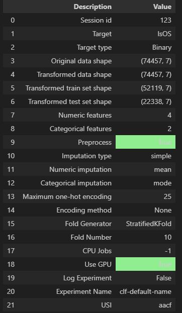
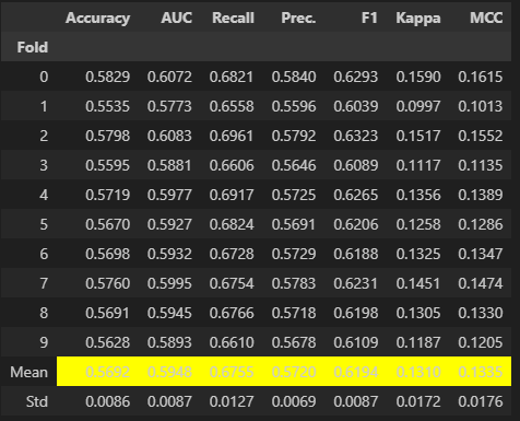
以下は、compare関数 で各モデルの学習を行った結果です。評価指標には precisionを取っています。(これについては、データが均衡になるよう設定し、正確なモデル予測精度を計測したかったためです。)
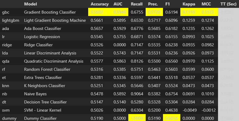
Accuracy、Precision 共に60%を割っているため精度がいいとは言えません。
次は、パラメータチューニングを行います。現状最適なモデルは Accuracy、Precision 共に最高値を叩き出している Gradient Boosting Classifier であるため、このモデルを調整します。
以下はその結果になります。
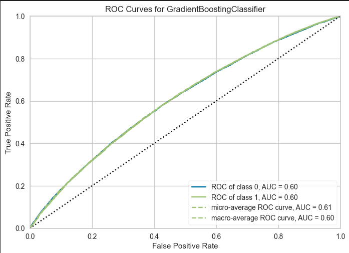
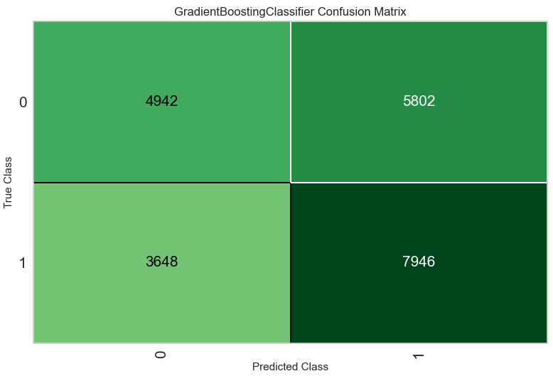
何故か調整後の方が精度が悪化しました。(何故?)評価結果として、精度が60%を割っていたため正確な分類は出来ていないといえます。
6. 議論
論文からは、以下のような予測に関する結果が得られています。
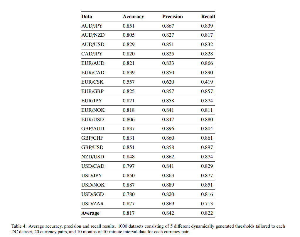
しかし、原論文ではデータセットの生成に使用する閾値を0.010%, 0.013%, 0.015%, 0.018% and 0.020%に限定しており、そこから最適な閾値を選択していました。
0.010%と0.02%の閾値を用いたデータセットにおける 目的変数の均衡性 を、今回作者が作成したデータセットと比較するため棒グラフで説明します。
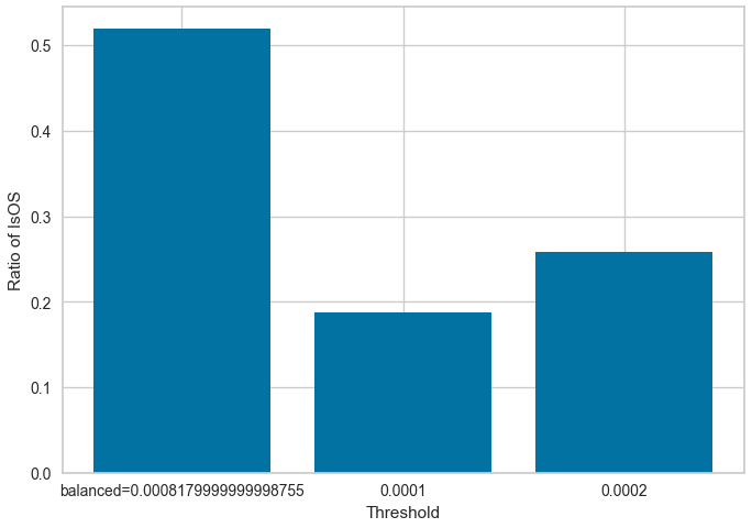
論文で示されている閾値を用いると、平均して 20~25% 程度しかOSイベントを持っていないことが分かります。そのため、不均衡データを用いた判別モデルによる評価結果ということが分かりました。
このことから、作者が作成した判別モデルの精度と論文の判別モデルの精度に差が生じた要因の一つとして、データセットの均衡性 が原因と推測します。
また遺伝的プログラミングを用いた予測に関しても同様だと考えています。DC-OSデータセットはその性質上、閾値を小さくするほどDCイベントやOSイベントの長さが短くなります。そのため、閾値が小さいほどイベントの長さのボラリティが小さい ことから予測が容易になると考えられます。
以下の図は閾値ごとのイベントの長さを箱ひげ図で表したものです。外れ値は除外しています。
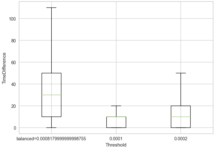
これらが要因となり、判別モデルと遺伝的プログラミングを用いた予測モデルの精度が向上しなかったと考えられます。
まとめ
ここまで読んでくださり、ありがとうございます。
今回は趣向を変えて、深層学習を一切使用しない為替予測モデルの実装を行ってみました。大学の春休み中、為替予測モデルの論文を読み漁りましたが、lag-modelの何と多いことか…。ここまでくると、予測精度が高いモデル=lag-modelなのではと思うほど多かったです。(実装するのは楽しいですが)
今回も、データセットの不備という問題点が要因となり、高精度の為替予測モデルの開発は頓挫しました。しかし、OSイベントの長さがDCイベントの長さの平均2倍になるという性質は、実用性がありそうで面白いと感じました。
次は、深層学習を用いた為替予測モデルに立ち返り、未来の価格を予測するというアプローチから脱却し、別のアプローチからlag-modelを生じない高精度な予測モデルを実装したいと思います。
参考文献
遺伝的アルゴリズムと遺伝的プログラミングを自力で実装して理解する
A CNN-STLSTM-AM model for forecasting USD/RMB exchange rate
Welcome to gplearn’s documentation!
ESTIMATING DIRECTIONAL CHANGES TREND
REVERSAL IN FOREX USING MACHINE LEARNING