In this article, I'm going to introduce my new paper "Conditionally Whitened Generative Models For Probabilistic Time Series Forecasting" (https://arxiv.org/abs/2509.20928).
Introduction
First, I'm going to introcude the task, Probabilistic Time Series Forecasting. There are some definations:
$d$: Dimensionality of the time series
$T_h$: Historical sequence length
$T_f$: Forecast horizon
$\textbf{C}$: Historical observations, the shape is $\mathbb{R}^{d \times T_h}$
$\textbf{X}_0$: Future time series, the shape is $\mathbb{R}^{d \times T_f}$
The task of probabilistic time series forecasting (TSF) is to learn the distribution of future time series $\textbf{X}_0$ given the historical observations $\textbf{C}$, denoted as $P_{\textbf{X}_0|\textbf{C}}$.
Challenges
TSF and probabilistic TSF are extremely important for decision-making in various domains such as finance, healthcare, environmental science and transportation. But there are several challenges:
- $\textbf{Non-stationarity}$: Long-term trends, seasonality, and heteroscedasticity
- $\textbf{Complex inter-variable dependencies}$: Intricate correlations between variables
- $\textbf{Inherent data uncertainty}$: Short-term fluctuations and noise
- $\textbf{Distribution shift}$: Distribution shift between training and test data
Due to the 4 challenges, a generative model usually cannot estimate $P_{\textbf{X}_0|\textbf{C}}$ well. But several previous models have shown that prior models derived from $\textbf{C}$ can substantially improve the quality of diffusion models. (The term 'prior' here refers to an auxiliary model that estimates the conditional mean, conditional variance, or other numerical characteristics. It does not refer to other meanings of 'prior', such as physical constraints or similar concepts.) But some key questions about prior models are unanswered:
- How do priors models improve performance and what accurate should the prior models be?
- How to train such priors models effectively?
- Are existing prior-integration mechanisms redundant, and can they be simplified in diffusion frameworks?
A Theorem
To answer Q1, we should begin from the TV error bound of diffusion model. Let $P_{X|C}$ is true conditional distribution of $ X \in \mathbb{R}^{d_x} $ given $ C $. Let $\widehat{P}_{X|C}$ be the distribution estimated by a default diffusion model. When the total step of diffusion is fixed, the TV error bound of diffusion model is [Fu, 2024; Oko, 2023; Chen, 2023]:
$$
D_{TV}(P_{X|C}, \widehat{P}_{X|C})=K_1 \cdot \sqrt{ D_{KL}(P_{X|C}|| N(0,I_{d_x}) )} + K_2 \cdot \varepsilon_{dis} + K_3 \cdot \varepsilon_{score},
$$
where $K_{1,2,3}$ are constants, $\varepsilon_{dis}$ is the discretization error of SDE and $\varepsilon_{score}$ is the error of score matching. $N(0,I_{d_x})$ is the terminal distribution of the default diffusion model. Some previous works change $N(0,I_{d_x})$ by normal distributions parameterized by some prior models, and get substantial gain. E.g., [CARD, 2022], [TMDM, 2024] change $N(0,I_{d_x})$ into $N(\widehat{\mu}_{X|C},I_{d_x})$ and [NsDiff, 2025] changes $N(0,I_{d_x})$ into $N(\widehat{\mu}_{X|C},\widehat{\Sigma}_{X|C})$.
Let's take NsDiff as an example. When such replacement of terminal distribution can have gain in performance, i.e. $D_{KL}(P_{X|C}|| N(\widehat{\mu}_{X|C},\widehat{\Sigma}_{X|C}) ) \leq D_{KL}(P_{X|C}|| N(0,I_{d_x}) )$? Our theorem gives a sufficient condition:
$$
( \min_{i \in {1,\dots,d_x}} \widehat{\lambda}_{X|C,i} )^{-1}
( | \mu_{X|C} - \widehat{\mu}_{X|C} |_2^2 + | \Sigma_{X|C} - \widehat{\Sigma}_{X|C} |_N ) + \sqrt{d_x} | \Sigma_{X|C} - \widehat{\Sigma}_{X|C} |_F \leq | \mu_{X|C} |_2^2,
$$
where $| \cdot |_F$ is F norm and $| \cdot |_N$ is nuclear norm (the sum of singular values).
Some comments to Th1:
- $\textbf{Theoretical guarantee}$: the sufficient condition of reducing the KLD
- $\textbf{Reveal important factors}$: the accuracy of $\widehat{\mu}_{X|C}$ and $\widehat{\Sigma}_{X|C}$, and the scale of the minimum eigenvalue of $\widehat{\Sigma}_{X|C}$, and the magnitude of $\mu_{X|C}$
- $\textbf{The basis of loss function}$: tell us how to design the loss functions for learning $ \mu_{X|C}$ and $ \Sigma_{X|C}$
- $\textbf{Why such replacement is good for Prob TSF}$: Plenty of examples shows replacing $N(0,I_{d_x})$ with $N(\widehat{\mu}_{X|C},\widehat{\Sigma}_{X|C})$ may not work for tabular data, but the replacement works in time series data. That's because for non-stationary time series data, $| \mu_{X|C} |_2^2$ is very huge, while that of tabular data is not huge
Joint Mean–Covariance Estimator (JMCE)
The theorem tell us that the accuracy of $\widehat{\mu}_{X|C}$ and $\widehat{\Sigma}_{X|C}$ are important of the performance gain and naturally tell us how to train them -- just minimize the LHS of the sufficient condition. The true covariance of time series is extremely hard to learn, so we chose to learn the sliding-window covariance $\widetilde{\Sigma}_{\textbf{X}_0, t}, t = 1, \ldots, T_f$, which is an alternative of the true covariance. Such sliding-window structure is unique for time series.
Let a Non-stationary Transformer [Liu, 2022] be the backbone of our JMCE, outputing $\widehat{\mu}_{\textbf{X}|\textbf{C}}, \widehat{L}_{1 | \textbf{C}}, \ldots, \widehat{L}_{T_f | \textbf{C}}$, where $\widehat{\mu}_{\textbf{X}|\textbf{C}}$ is the estimator of conditional mean, and $\widehat{\Sigma}_{\textbf{X}_0,t |\textbf{C}}:=\widehat{L}_{t|\textbf{C}} \widehat{L}_{t|\textbf{C}}^{\top}$ is the estimators of $\widetilde{\Sigma}_{\textbf{X}_0, t}$, for $ t = 1, \ldots, T_f$. We aim to design a loss function to minimize $\mathcal{L}_2 := \mathbb{E} \left| \textbf{X}_0 -\widehat{\mu}_{\textbf{X}|\textbf{C}} \right|_2^2$, $\mathcal{L}_F := \mathbb{E} \sum_{t=1}^{T_f} \left| \widetilde{\Sigma}_{\textbf{X}_0, t} - \widehat{\Sigma}_{\textbf{X}_0,t |\textbf{C}} \right |_F$ and $\mathcal{L}_{\text{SVD}} := \mathbb{E} \sum_{t=1}^{T_f} \left| \widetilde{\Sigma}_{\textbf{X}_0, t} - \widehat{\Sigma}_{\textbf{X}_0,t |\textbf{C}} \right|_N $.
In Th1, the sufficient condition is also influenced by the minimum eigenvalues of $\widehat{\Sigma}_{\textbf{X}_0,t |\textbf{C}}, t = 1, \ldots, T_f$. Thus, we design a novel penalty term to force the minimum eigenvalue to stay from 0:
$$
\mathcal{R}_{\lambda_{\text{min}}} \big( \widehat{\Sigma}_{\textbf{X}_0,t |\textbf{C}} \big) := \sum_{i=1}^{d} \text{ReLU} \big( \lambda_{\text{min}} - \widehat{\lambda}_{\widehat{\Sigma}_{\textbf{X}_0,t |\textbf{C}},i} \big),
$$
where $\lambda_{\text{min}}$ is a hyperparameter and $\widehat{\lambda}_{\widehat{\Sigma}_{\textbf{X}_0,t |\textbf{C}},i} (i = 1, \ldots, d)$ denote the eigenvalues of $\widehat{\Sigma}_{\textbf{X}_0,t |\textbf{C}}$. Any eigenvalue smaller than $\lambda_{\min}$ will be penalized. Finally, the loss function of JMCE is:
$$
\mathcal{L}_{\text{JMCE}} = \mathcal{L}_{2} + \mathcal{L}_{\text{SVD}} + \lambda_{\text{min}} \sqrt{d \cdot T_f} \mathcal{L}_{F} + w_{\text{Eigen}} \cdot \sum_{t=1}^{T_f} \mathcal{R}_{\lambda_{\text{min}}} \left( \widehat{\Sigma}_{\textbf{X}_0,t |\textbf{C}} \right),
$$
where $w_{\text{Eigen}}$ is a hyperparameter that controls the strength of the penalty.
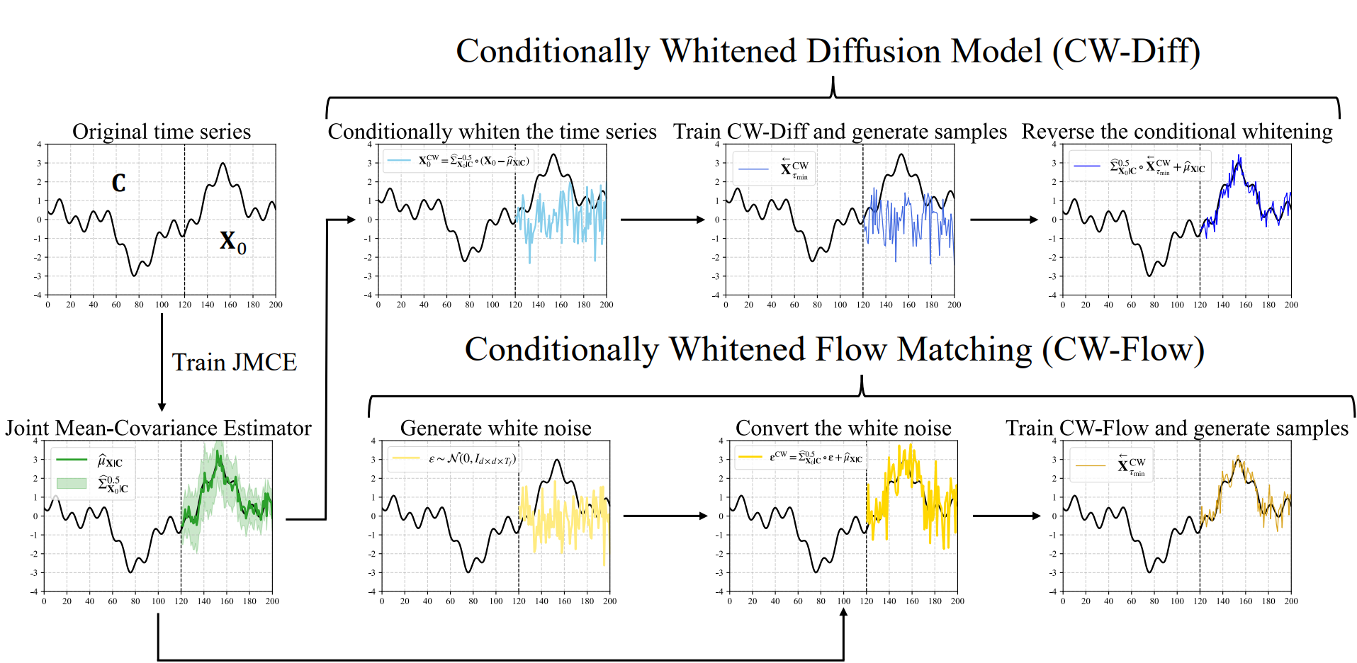
Condtionally Whitened Diffusion Models (CW-Diff) and Condtionally Whitened Flow Matching (CW-Flow)
For simplicity, we define $\widehat{\Sigma}^k_{\textbf{X}_0 |\textbf{C}} := [ \widehat{\Sigma}^k_{\textbf{X}_0,1 |\textbf{C}}, \ldots, \widehat{\Sigma}^k_{\textbf{X}_0,T_f |\textbf{C}} ] \in \mathbb{R}^{d \times d \times T_f}$
for $k \in {-0.5, 0.5}$ and $\mathbf{\epsilon} := [\epsilon_1, \ldots, \epsilon_{T_f}] \in \mathbb{R}^{d \times T_f}$.
We define the tensor operation
$$
\widehat{\Sigma}^{0.5}_{\textbf{X}_0 |\textbf{C}} \circ \mathbf{\epsilon}
:= [ \widehat{\Sigma}^{0.5}_{\textbf{X}_0,1 |\textbf{C}} \cdot \epsilon_1, \ldots,
\widehat{\Sigma}^{0.5}_{\textbf{X}_0,T_f |\textbf{C}} \cdot \epsilon_{T_f} ]
\in \mathbb{R}^{d \times T_f}.
$$
Accordingly, we say that a tensor follows $\mathcal{N}(\widehat{\mu}_{\textbf{X}|\textbf{C}}, \widehat{\Sigma}_{\textbf{X}_0 |\textbf{C}})$ if it has the same distribution as
$\widehat{\Sigma}^{0.5}_{\textbf{X}_0 |\textbf{C}} \circ \mathbf{\epsilon} + \widehat{\mu}_{\textbf{X}|\textbf{C}}$.
CW-Diff
With the previous definition, we can use an OU process with drift and covariance to diffuse the original time series $\textbf{X}_0$ to $\mathcal{N}(\widehat{\mu}_{\textbf{X}|\textbf{C}}, \widehat{\Sigma}_{\textbf{X}_0 |\textbf{C}})$:
$$
d \big( \textbf{X}_\tau - \widehat{\mu}_{\textbf{X}|\textbf{C}} \big)
= - \tfrac{1}{2} \beta_\tau \big( \textbf{X}_\tau - \widehat{\mu}_{\textbf{X} | \textbf{C}} \big) d \tau
+ \sqrt{\beta_\tau} \cdot \widehat{\Sigma}^{0.5}_{\textbf{X}_0 |\textbf{C}} \circ d \textbf{W}_\tau,
\ \textbf{X}_0 \sim P_{\textbf{X} | \textbf{C}},
$$
for $\tau \in [0,1]$ and $\textbf{W}_\tau$ is a Brownian motion in $\mathbb{R}^{d \times T_f}$.
Furthermore, the following SDE is equivalent to upper SDE:
$$
d \ \widehat{\Sigma}^{-0.5}_{\textbf{X}_0 |\textbf{C}} \circ \big( \textbf{X}_\tau - \widehat{\mu}_{\textbf{X}|\textbf{C}} \big) = - \tfrac{1}{2} \beta_\tau \cdot \widehat{\Sigma}^{-0.5}_{\textbf{X}_0 |\textbf{C}} \circ \big( \textbf{X}_\tau - \widehat{\mu}_{\textbf{X}|\textbf{C}} \big) d \tau + \sqrt{\beta_\tau} d \textbf{W}_\tau, \ \tau \in [0,1],
$$
which implies that the diffusion processes can be directly performed on $\textbf{X}^{\text{CW}}_0 := \widehat{\Sigma}_{\textbf{X}_0 |\textbf{C}}^{-0.5} \circ \big( \textbf{X}_0 - \widehat{\mu}_{\textbf{X}|\textbf{C}} \big)$. We call this operation conditional whitening (CW).
The CW operation subtracting $\widehat{\mu}_{\textbf{X}|\textbf{C}}$ and de-correlate every time point in $\textbf{X}_0$ given $\textbf{C}$, eliminating the non-stationary components and simplifying the inter correlation. And the forward process of CW-Diff has the same form with DDPM:
$$
d \textbf{X}^{\text{CW}}_\tau = - \tfrac{1}{2} \beta_\tau \textbf{X}^{\text{CW}}_\tau d \tau + \sqrt{\beta_\tau } d \textbf{W}_\tau , \ \tau \in [0,1],
$$
which remains the diffusion processes simple. The loss function and the reverse process is same with DDPM. Assume the final sample generated by reverse process is $\overset{\leftarrow}{\textbf{X}}{}^{\text{CW}}_{\tau_\text{min}}$ ($\tau_\text{min}$ is the early stopping time), we just need to reverse the CW operation:
$$
\overset{\leftarrow}{\textbf{X}}_{\tau_\text{min}} = \widehat{\Sigma}_{\textbf{X}_0|\textbf{C}}^{0.5} \circ \overset{\leftarrow}{\textbf{X}}{}^{\text{CW}}_{\tau_\text{min}} + \widehat{\mu}_{\textbf{X}|\textbf{C}},
$$
and we get the sample approximates $P_{\textbf{X}|\textbf{C}}$.
CW-Flow
In CW-Diff, the inverse matrices of $\widehat{\Sigma}_{\textbf{X}_0,t |\textbf{C}}$ need to be computed, with a complexity of $\mathcal{O}(d^3 T_f)$. To reduce this cost and improve efficiency, we transition to the Flow Matching framework.
\vspace{1em}
Compared to the original flow matching, our Conditionally Whitened Flow Matching (CW-Flow) just changes the terminal distribution.
Experimental Results
We use CRPS, QICE, Prob-Correlation score, Conditional FID to evaluate the default generative models and CW-ed generative models. We conduct experiments on 5 datasets, and on 6 generative models: [TimeDiff, 2023], [SSSD, 2023], [Diffusion-TS, 2024], [TMDM, 2024], [NsDiff, 2025], [FlowTS, 2025]. A general result is:
| Dataset | Win rate of CW-Gen |
|---|---|
| ETTh1 | 22/24 ≈ 91.67% |
| ETTh2 | 22/24 ≈ 91.67% |
| ILI | 21/24 ≈ 87.50% |
| Weather | 22/24 ≈ 91.67% |
| Solar Energy | 19/24 ≈ 79.17% |
"Win" means a CW-Gen model overperform a default generative model on one metric. Since we have 4 metrics and 6 kinds of generative models, we have 24 sets of experiments on each datasets.

In the first dimension, CW-Gen fits better. In the second dimension, the distribution shift is mitigated.
Conclusion
- $\textbf{CW-Gen Framework}$: Proposed a unified conditional generation framework $\textbf{CW-Gen}$ with two instantiations—$\textbf{CW-Diff}$ and $\textbf{CW-Flow}$
- $\textbf{Theoretical Support}$: Provided \textbf{sufficient conditions} to guarantee the improvement of CW-Gen
- $\textbf{JMCE}$: Designed Joint Mean–Covariance Estimator ($\textbf{JMCE}$) to estimate the conditional mean and sliding-window covariance jointly, and control the minimum eigenvalues simultaneously
- $\textbf{Empirical Results}$: Integrated CW-Gen with $\textbf{6 SOTA generative models; tested on 5 real datasets}$. The results confirm better capture of non-stationarity, improved modeling of inter-variable dependencies, higher sample quality, and better mitigation of distribution shifts