SAS Viyaによる基本的な予測モデリングデモを体験する流れ

SAS ViyaはAIプラットフォームを提供しています。デモもあるのですが、全体が英語なので利用するまでに躊躇してしまう人も多いかと思います。そこで、Pythonで基本的な予測モデリングデモを体験するまでの流れを紹介します。

利用開始まで

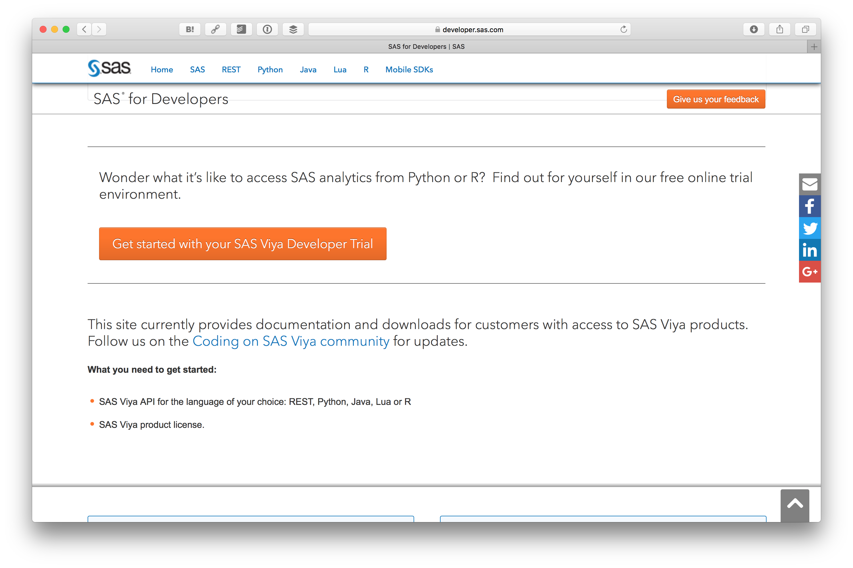
まず SASの開発者サイトにアクセスします。開発者サイトは https://developer.sas.com/home.html です。

そして、 Get started with your SAS Viya Developer Trial を押します。

試すためには SAS Profile （SASプロファイル） というのが必要です。まず Create one をクリックします。

SASプロファイルを登録するをクリックします。

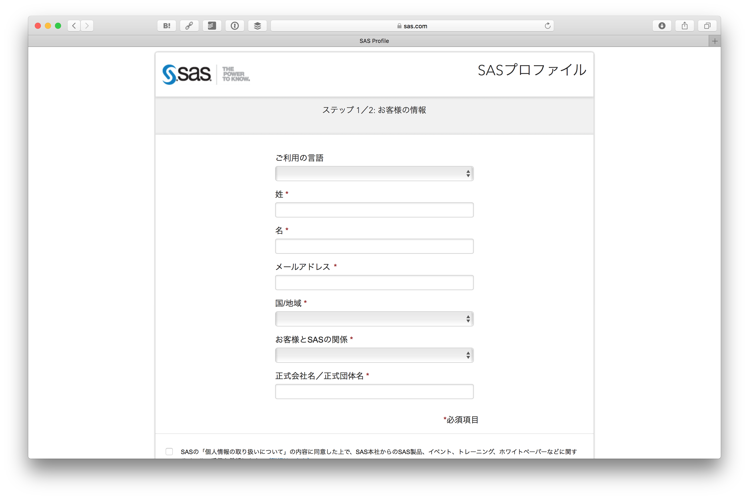
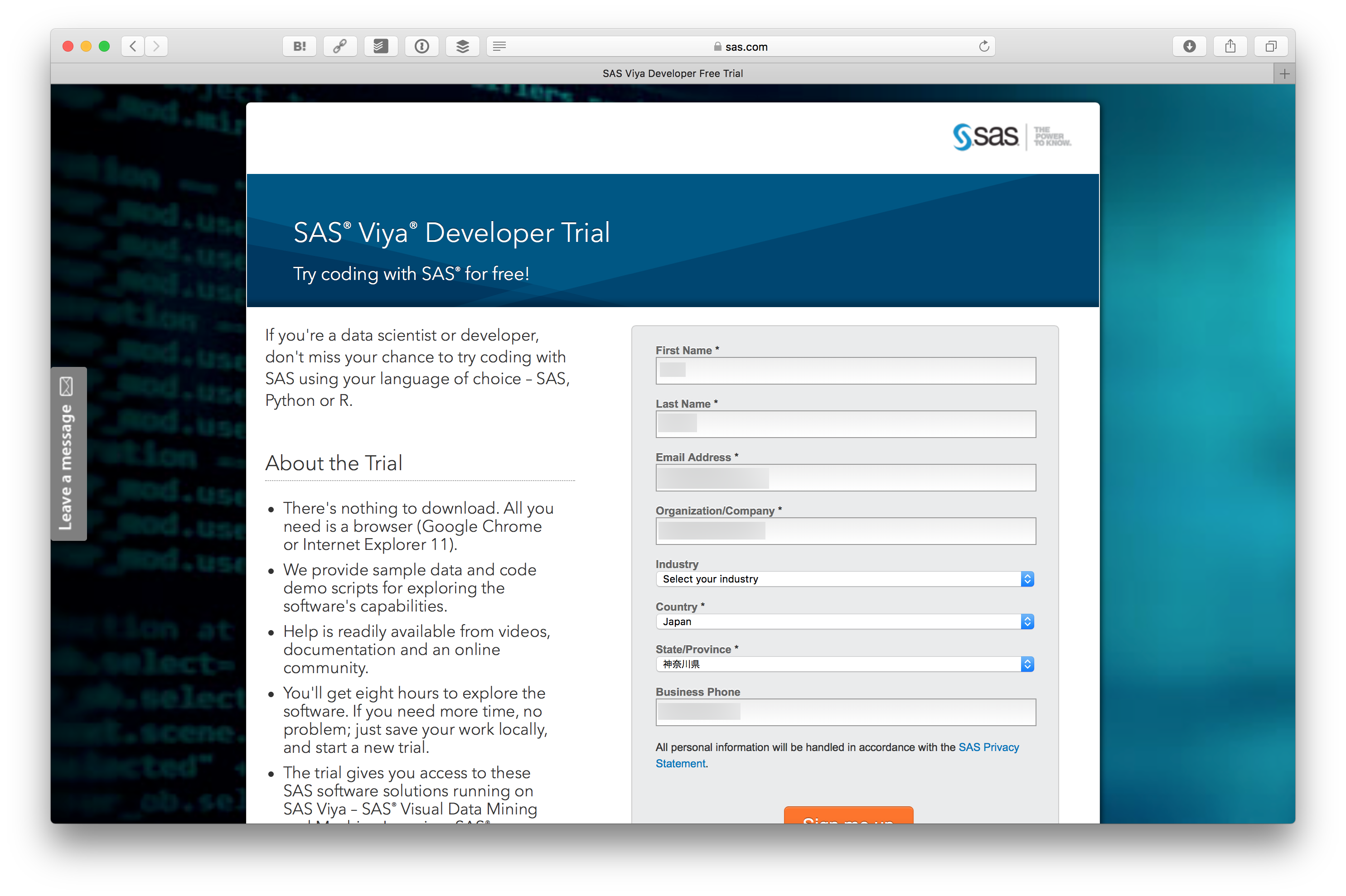
情報を入力します。

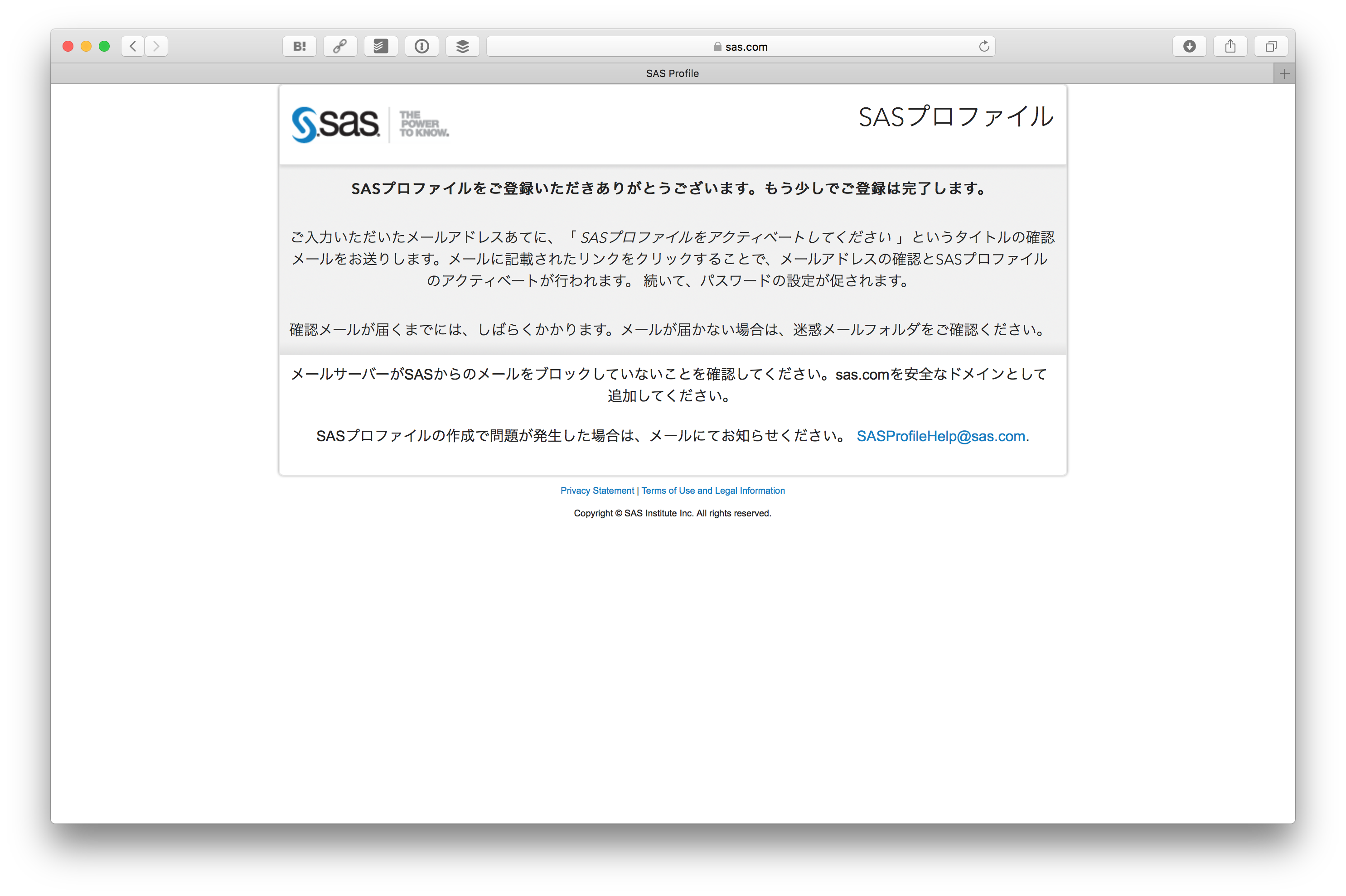
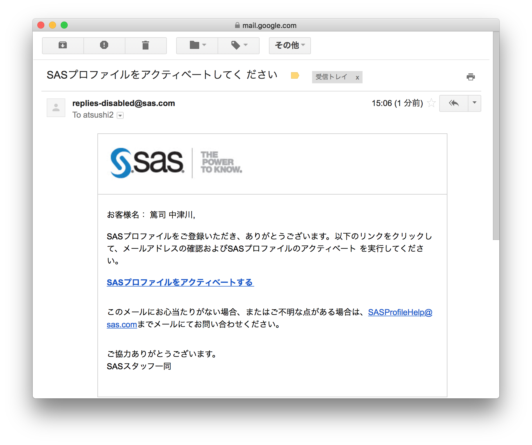
フォームを送信するとメールが送られてきます。

メールに書かれている SASプロファイルをアクティベートする をクリックします。

そしてパスワードを設定します。

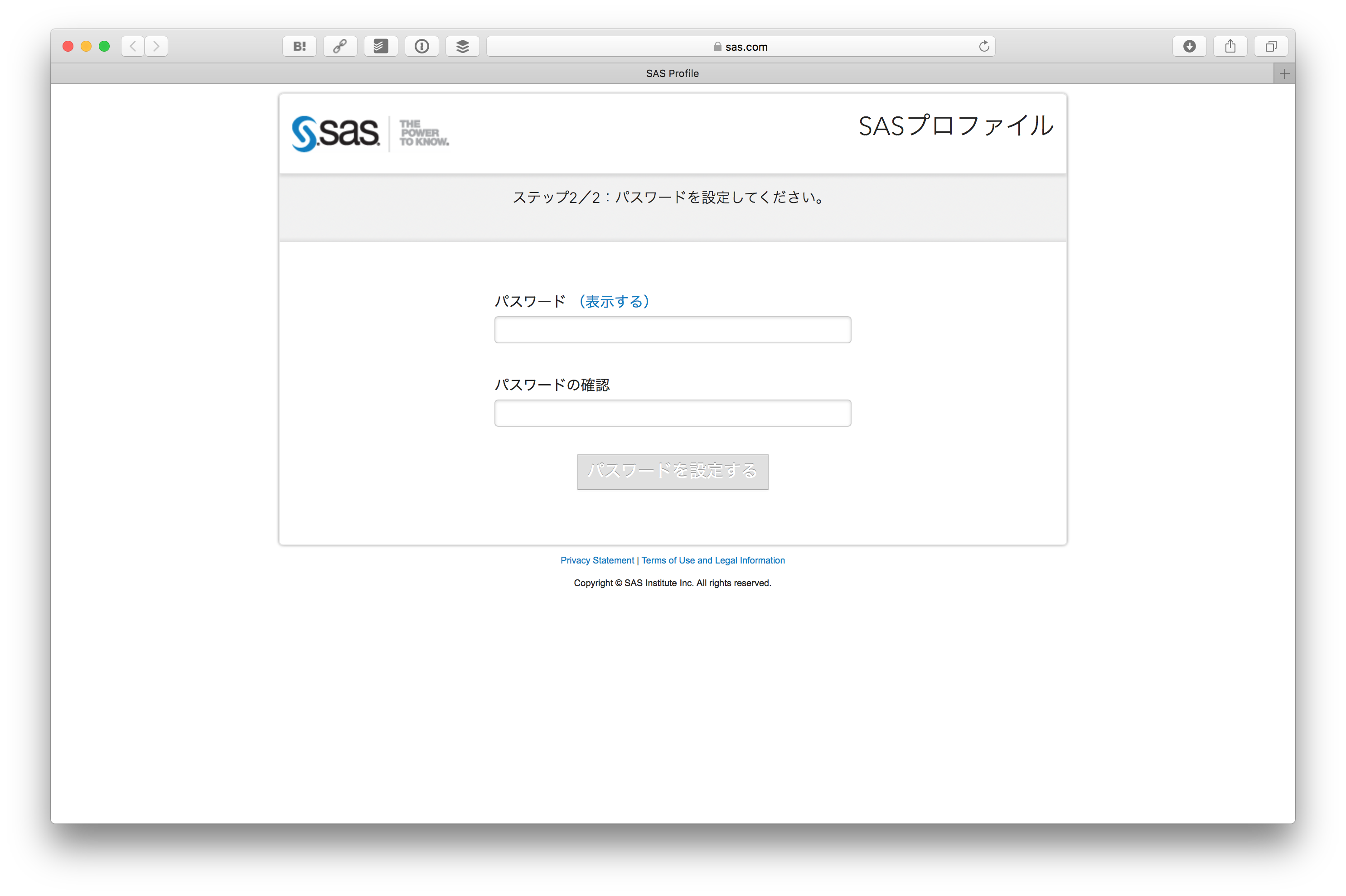
SASプロファイルがアクティベートされます。 続ける をクリックします。

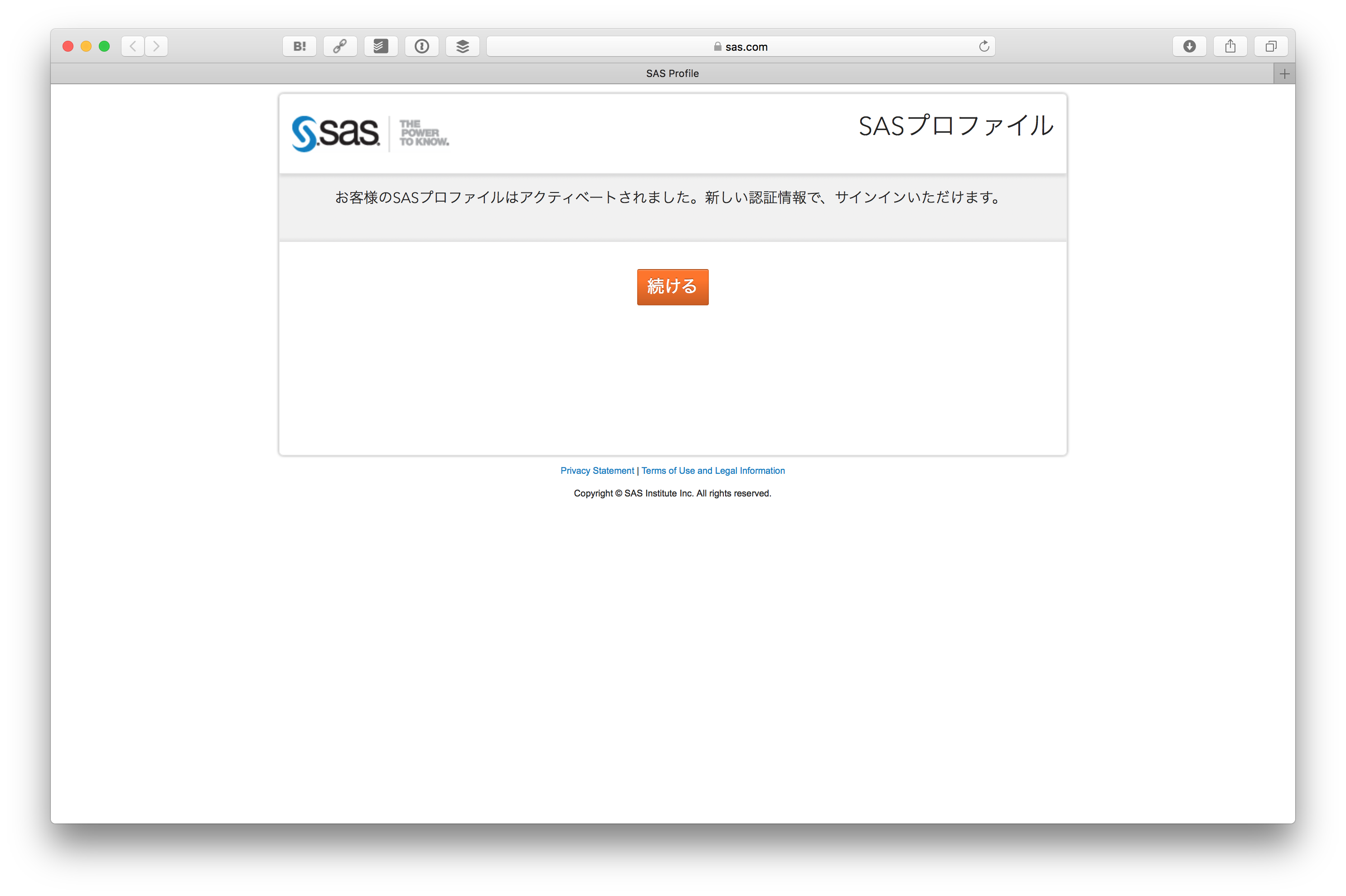
そうすると先ほどの SAS® Viya® Developer Trial の画面に戻ってきますので、 今度はSign In をクリックします。

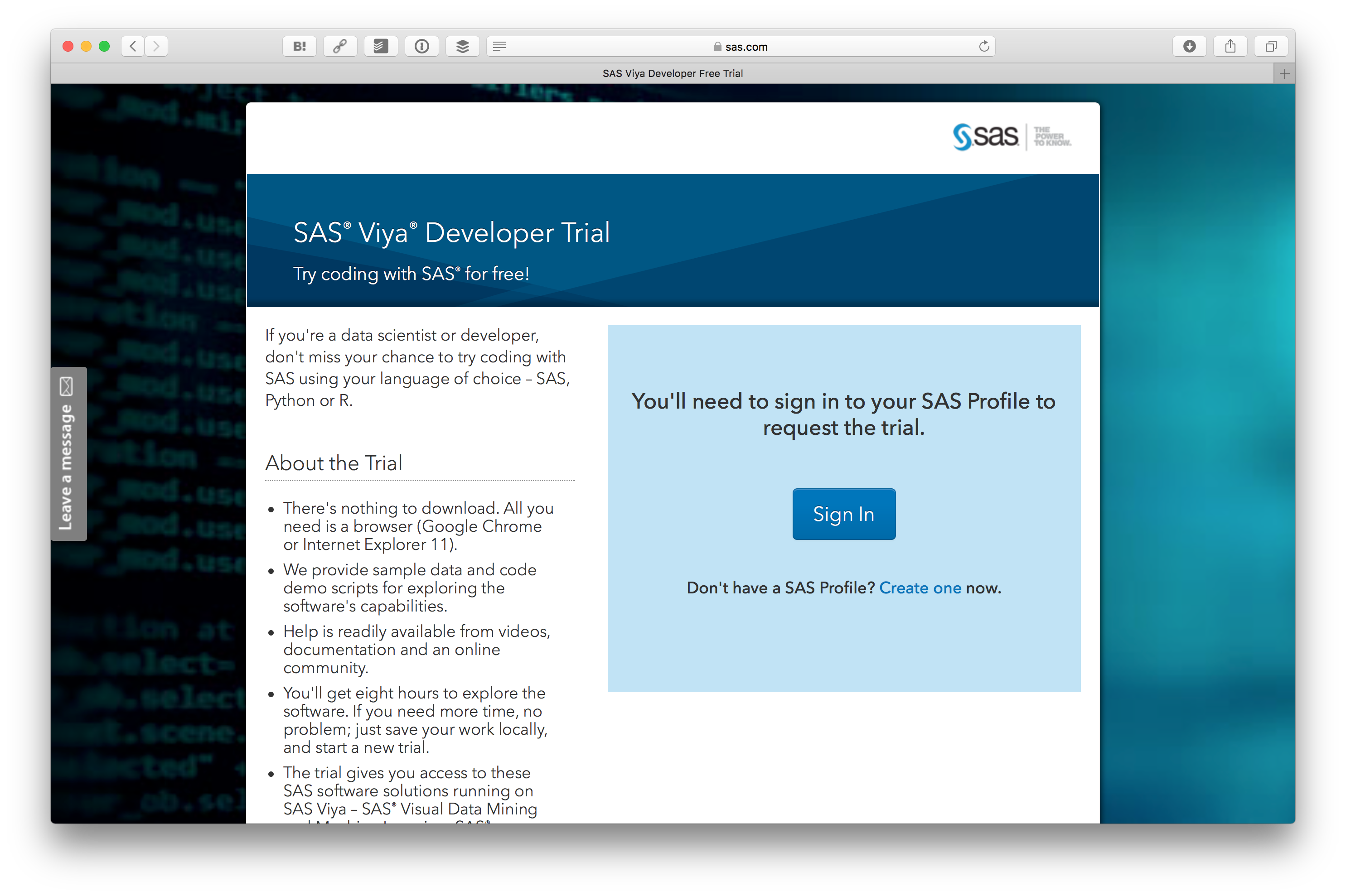
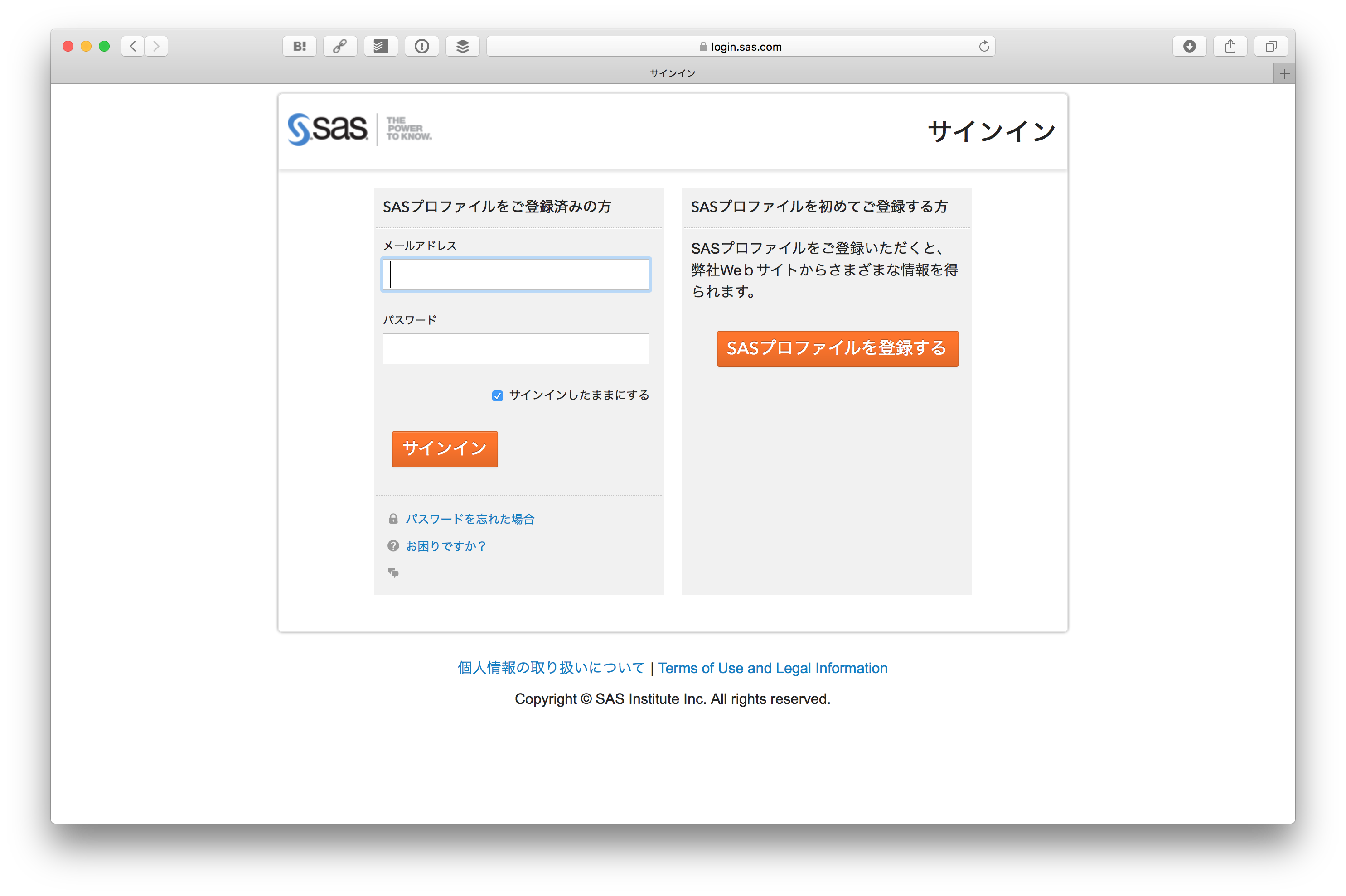
先ほど登録したSASプロファイルのID、パスワードでログインします。

ログインすると SAS® Viya® Developer Trial の画面に戻ってきますが、今回はプロファイルの内容が入力されているはずです。一番下にある Sign me upボタンをクリックします。

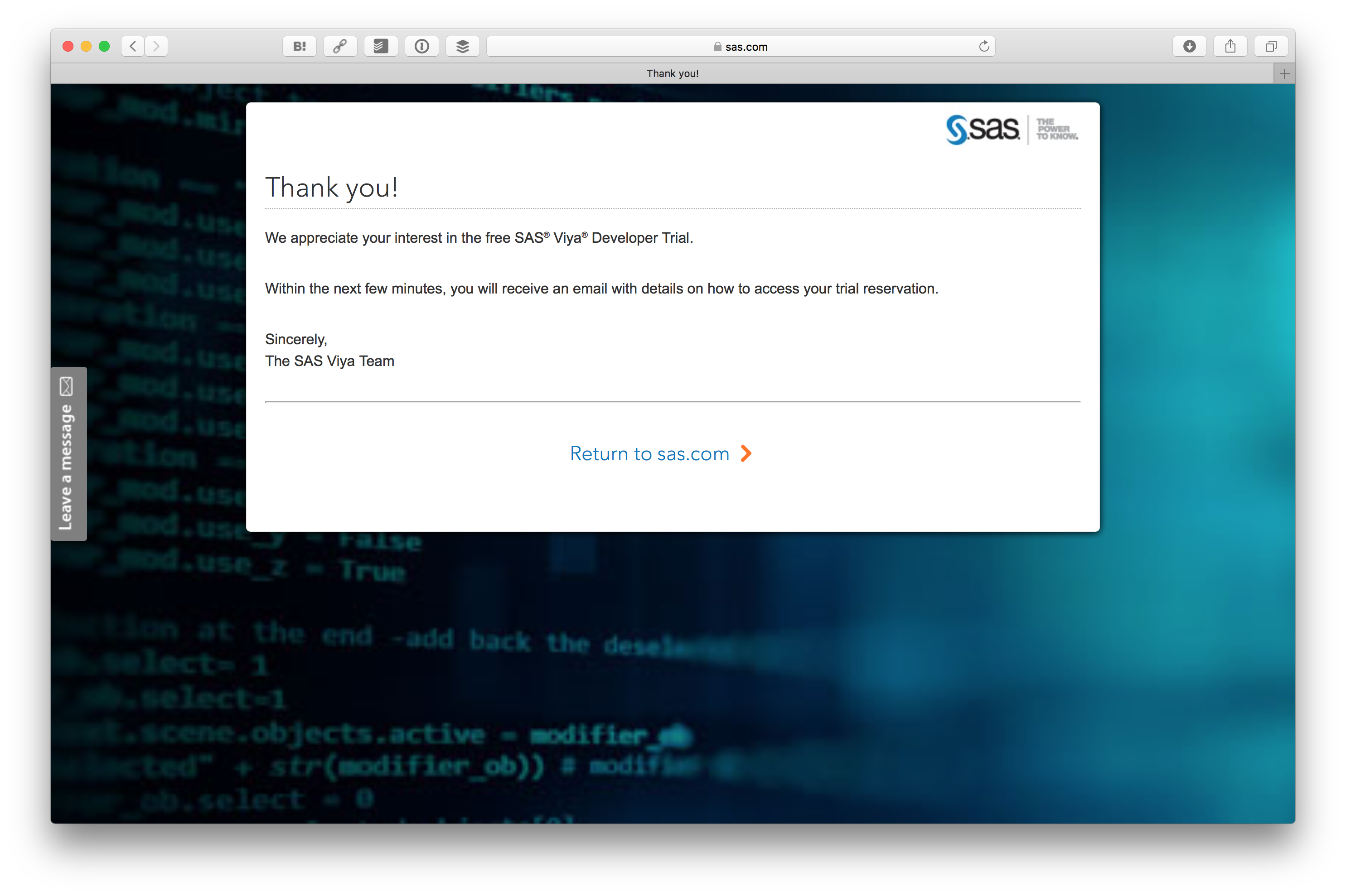
これで SAS® Viya® Developer Trial の申し込みが終わりました。数分後にメールが送られてきます。

送られてきたメールにある Log in to your Trial Portal のリンクをクリックします。

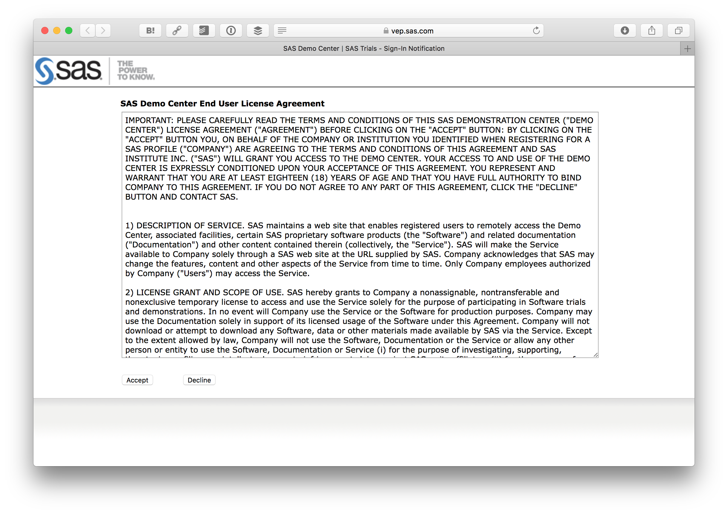
利用規約が表示されますので、問題なければAcceptボタンを押します。

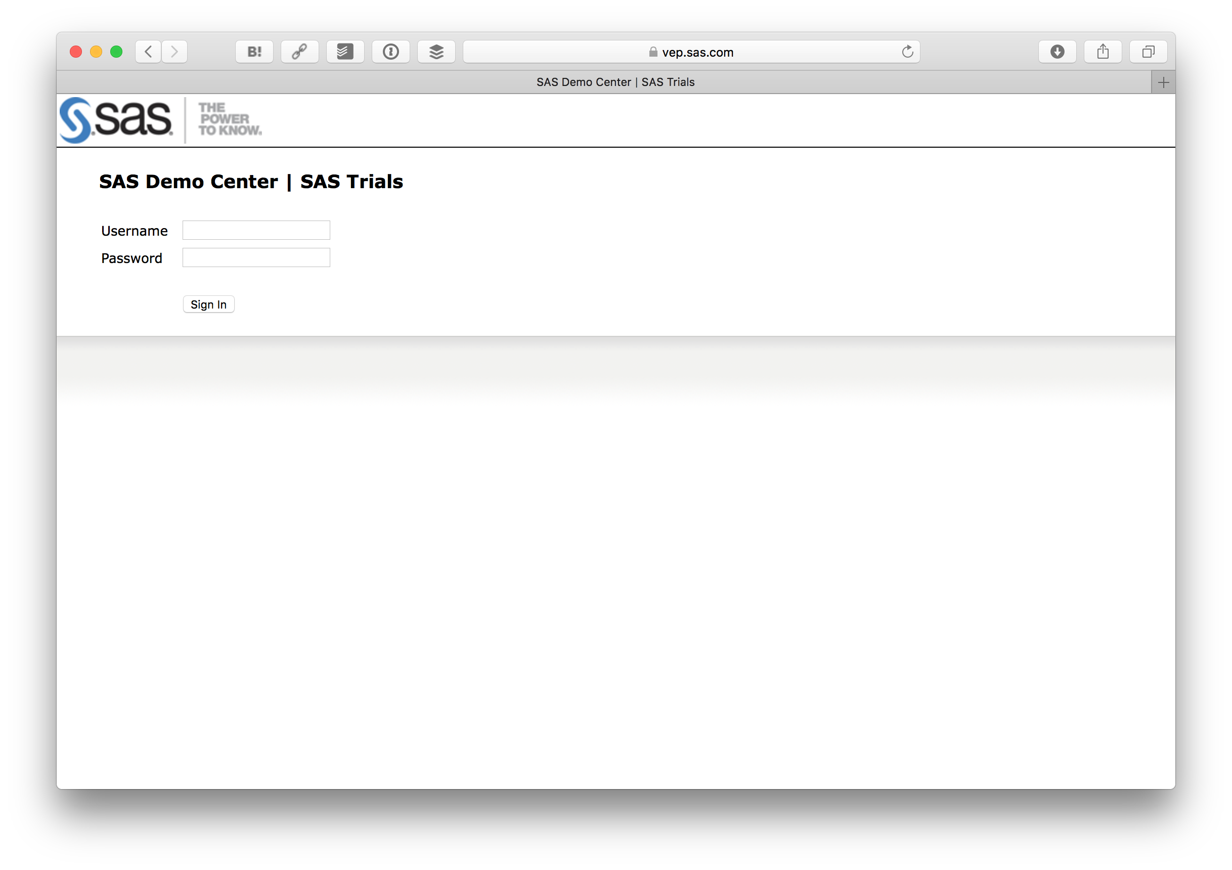
そうするとログインフォームが出るので、先ほど登録したID、パスワードでログインします。

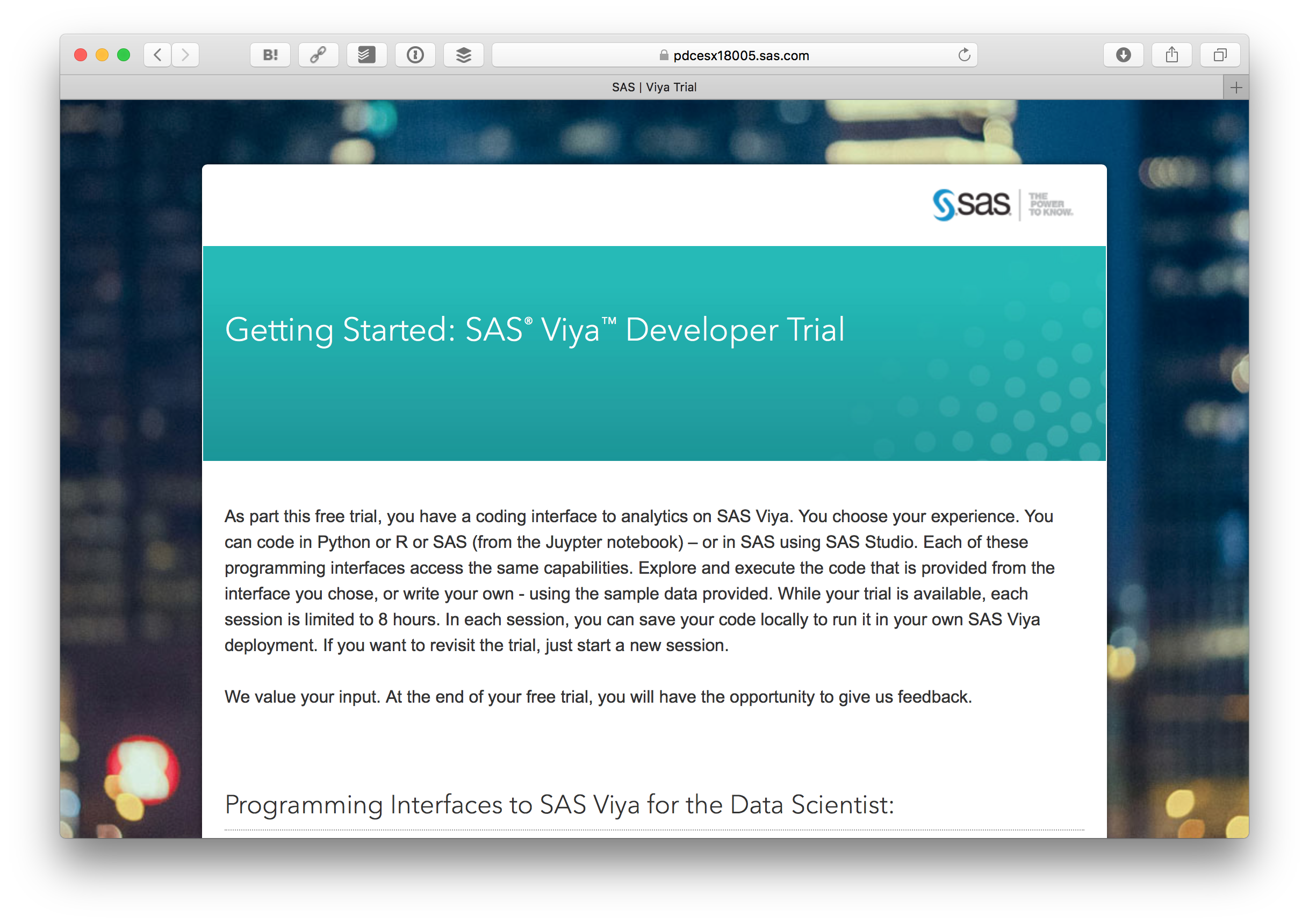
ログインすると Getting Started: SAS® Viya™ Developer Trial が表示されます。

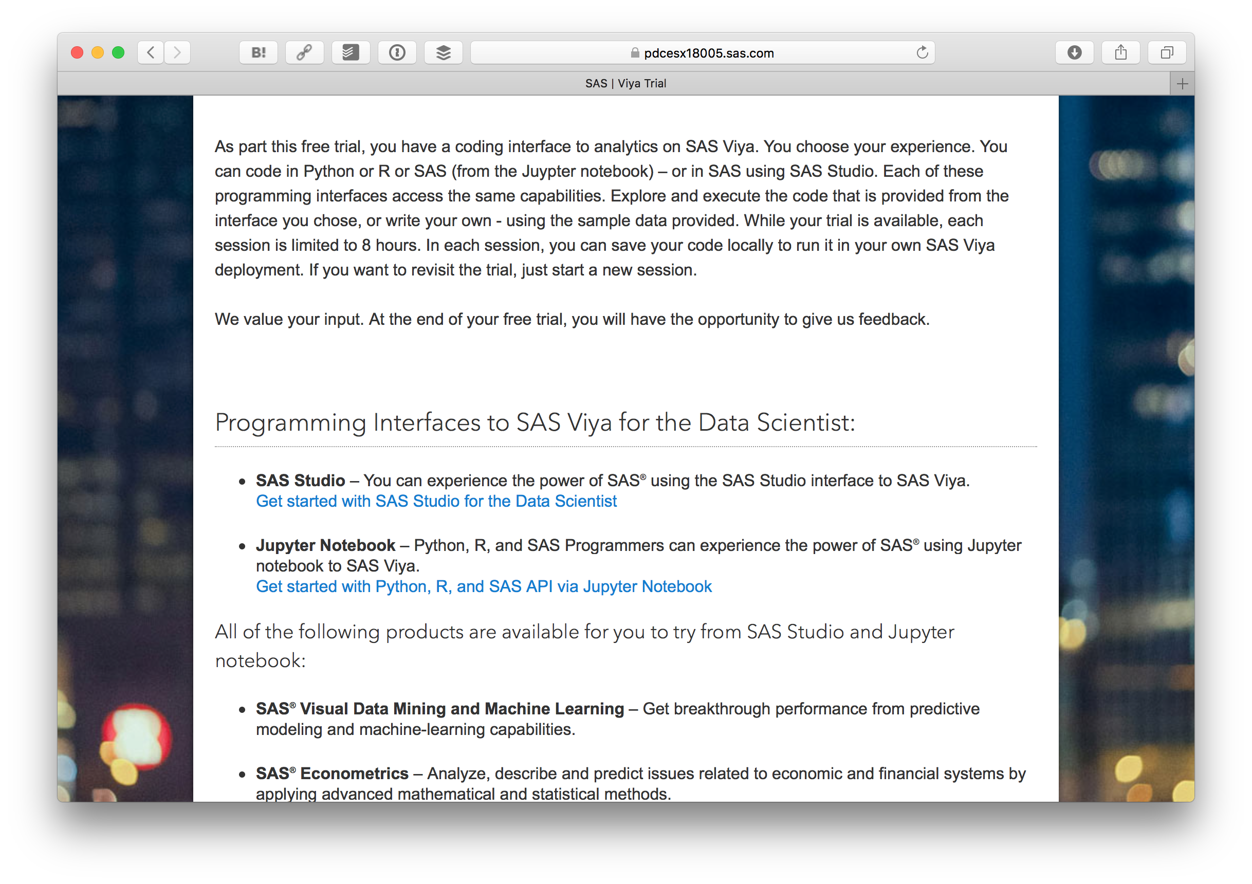
下の方にある Get started with Python, R, and SAS API via Jupyter Notebook をクリックします。

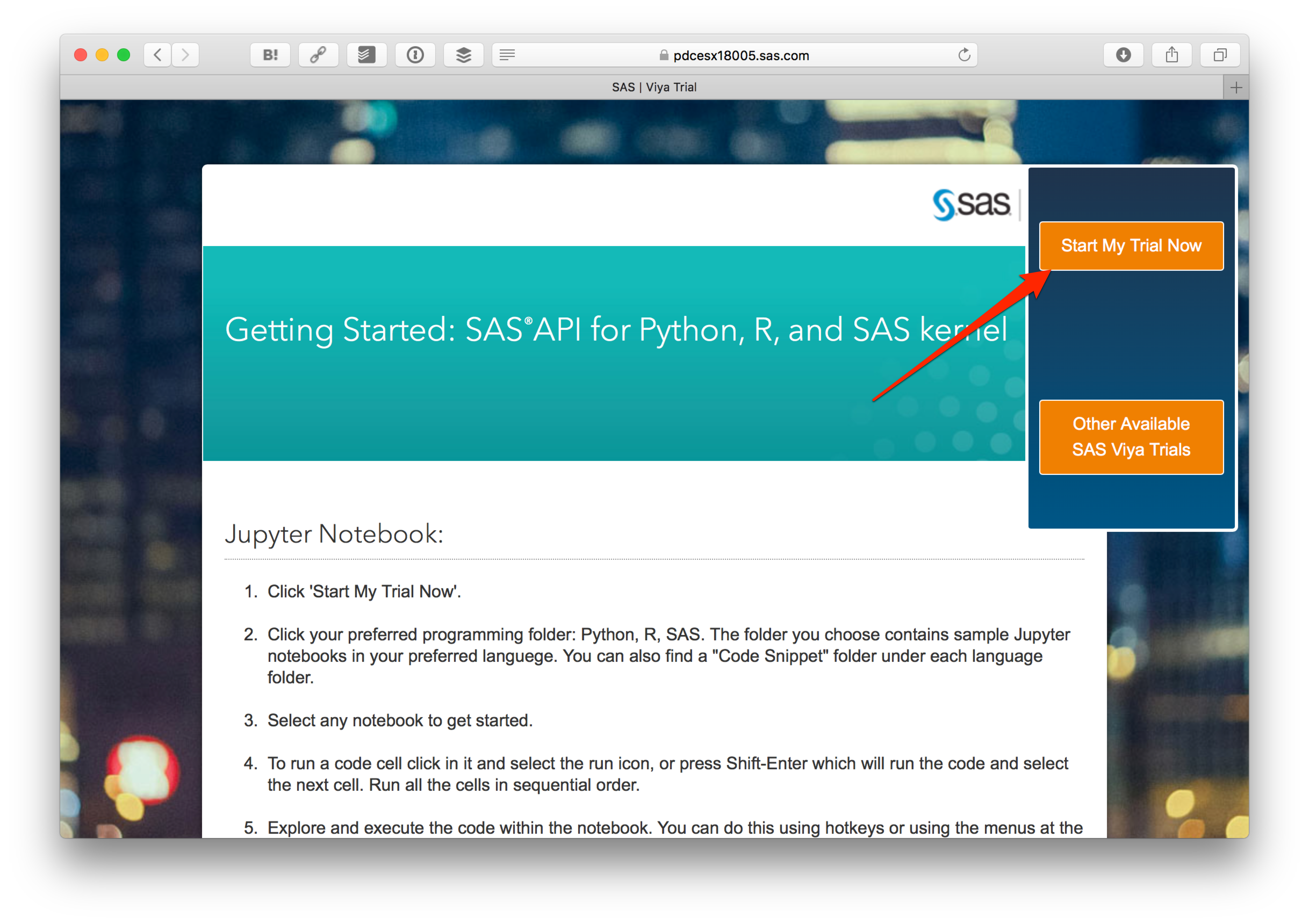
さらに Start My Trial Now をクリックします。

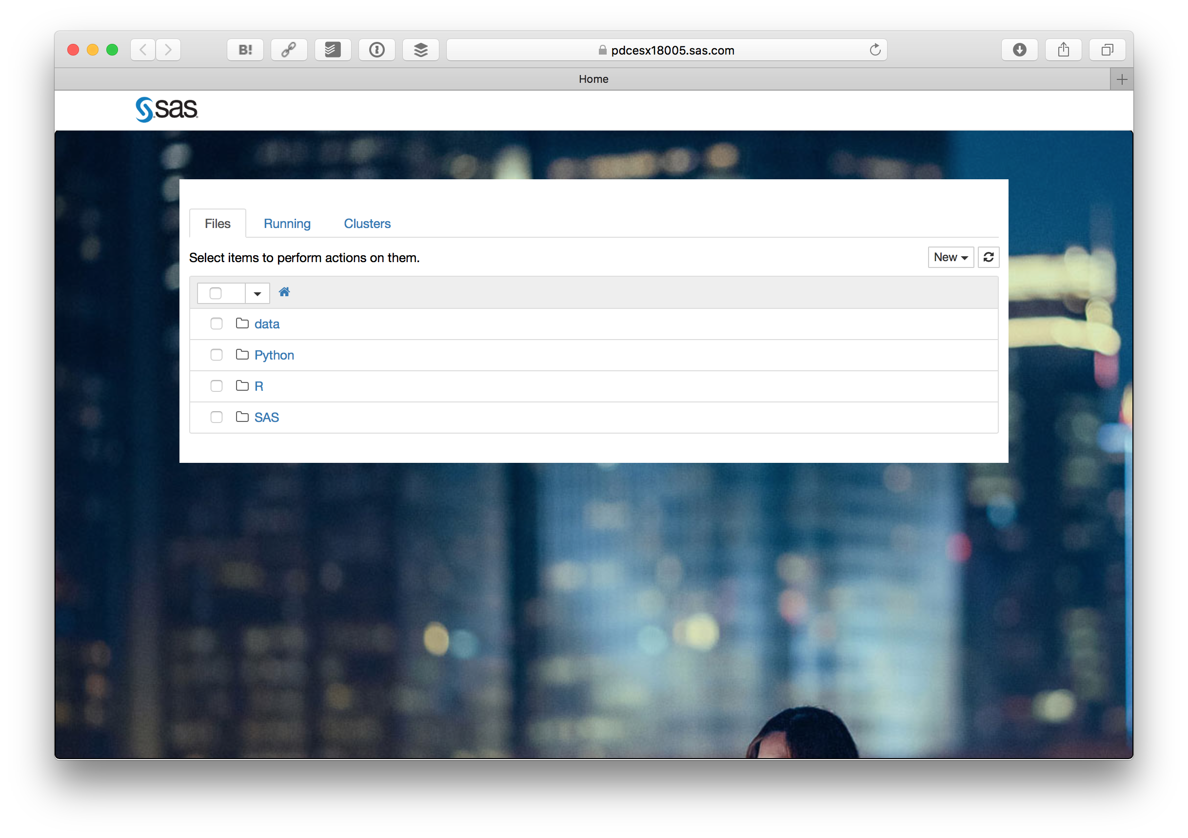
そうすると見慣れたJupyter Notebookの画面が出ます。Pythonフォルダの中にある Basic Predictive Modeling Example.ipynb をクリックします。

---

ここからは Basic Predictive Modeling Example.ipynb に書かれている内容の意訳です。英語の後に日本語を参考として載せています。

Overview（概要）

This is a simple end to end example of how you can use SAS Viya for analysis

これは分析のためにSAS Viyaを使用する方法の簡単な例です。

The example follows these steps:

この例は以下の手順に沿って行います。

1. Importing the needed Python packages（必要なPythonパッケージをインポートする）
2. Starting a CAS session on an already running CAS server（実行中のCASサーバでCASセッションを開始する）
3. Checking the server status（サーバの状態を確認する）
4. Loading data from the local file system to the CAS server（ローカルファイルからCASサーバへのデータの読み込み）
5. Explore the data（データを調べる）
6. Impute missing values（欠損値の代入）
7. Partition the data into training and validation partitions（データをパーティション（トレーニングパーティションと検証）に分割する）
8. Build a decision tree（ディシジョンツリーを構築する）
9. Build a neural network（ニューラルネットワークを構築する）
10. Build a decision forest（ディシジョンフォレストを構築する）
11. Build a gradient boost（Gradient Boostingを作成する）
12. Assess the models（モデルを評価する）
13. Build ROC charts（ROCチャートを作成する）

Setup and initialize（セットアップと初期化）

Find doc for all the CAS actions here

CASアクションのドキュメントについてはこのドキュメントを見てください。
両方でターゲット変数の
In this code we import the needed packages and we assign variables for the modeling details that will be used later in the analysis

このコードでは、必要なパッケージをインポートし、解析の後半で使用されるモデリング用の変数を割り当てます。

from swat import *
from swat.render import render_html
from pprint import pprint
from matplotlib import pyplot as plt
import pandas as pd
import sys
%matplotlib inline

target          = "bad"
class_inputs    = ["reason", "job"]
class_vars      = [target] + class_inputs
interval_inputs = ["im_clage", "clno", "im_debtinc", "loan", "mortdue", "value", "im_yoj", "im_ninq", "derog", "im_delinq"]
all_inputs      = interval_inputs + class_inputs

indata_dir = '../data'
indata = 'hmeq'

Start CAS session（CASセッションの開始）

In this code we assign values for the cashost, casport, and casauth values. These are then used to establish a CAS session named sess.

このコードでは cashost、casportおよびcasauthに値を割り当てます。 これらは、 sess という名前のCASセッションを確立するために使用します。

cashost='localhost'
casport=5570
casauth='~/.authinfo'
sess = CAS(cashost, casport, authinfo=casauth, caslib="casuser")

# Load the needed action sets for this example:
# このデモで必要なアクションセットをロードします：
sess.loadactionset(actionset="dataStep")
sess.loadactionset(actionset="dataPreprocess")
sess.loadactionset(actionset="cardinality")
sess.loadactionset(actionset="sampling")
sess.loadactionset(actionset="regression")
sess.loadactionset(actionset="decisionTree")
sess.loadactionset(actionset="neuralNet")
sess.loadactionset(actionset="svm")
sess.loadactionset(actionset="astore")
sess.loadactionset(actionset="percentile")

Load data into CAS（CASにデータを読み込む）

if not sess.table.tableExists(table=indata).exists:
    indata = sess.upload_file(indata_dir+"/"+indata+".csv", casout={"name":indata})

Explore and Impute missing values（データの探索および欠損値の代入）

sess.summary(indata)

Explore data and plot missing values（データの探索および欠損値の確認）

sess.cardinality.summarize(
  table=indata, 
  cardinality={"name":"data_card", "replace":True}
)

tbl_data_card=sess.CASTable('data_card')
tbl_data_card.where='_NMISS_>0'
print("Data Summary".center(80, '-')) # print title
tbl_data_card.fetch() # print obs

tbl_data_card.vars=['_VARNAME_', '_NMISS_', '_NOBS_']
allRows=20000  # Assuming max rows in data_card table is <= 20,000
df_data_card=tbl_data_card.fetch(to=allRows)['Fetch']
df_data_card['PERCENT_MISSING']=(df_data_card['_NMISS_']/df_data_card['_NOBS_'])*100

tbl_forplot=pd.Series(list(df_data_card['PERCENT_MISSING']), index=list(df_data_card['_VARNAME_']))
ax=tbl_forplot.plot(
  kind='bar', 
  title='Percentage of Missing Values'
)
ax.set_ylabel('Percent Missing')
ax.set_xlabel('Variable Names');

Impute missing values（欠損値の代入）

r=sess.dataPreprocess.transform(
  table=indata,
  casOut={"name":"hmeq_prepped", "replace":True},
  copyAllVars=True,
  outVarsNameGlobalPrefix="IM",
  requestPackages=[
    {"impute":{"method":"MEAN"}, "inputs":{"clage"}},
    {"impute":{"method":"MEDIAN"}, "inputs":{"delinq"}},
    {"impute":{"method":"VALUE", "valuesContinuous":{2}}, "inputs":{"ninq"}},
    {"impute":{"method":"VALUE", "valuesContinuous":{35.0, 7, 2}}, "inputs":{"debtinc", "yoj"}}
  ]
)
render_html(r)

Partition data into Training and Validation（トレーニングと検証用パーティションにデータを投入）

The stratified action in the sampling actionset allows us to create two partition and observe the reponse rate of the target variable bad in both training and validation

サンプルデータのアクションセットにある階層化されたアクションで2つのパーティションを作成します。トレーニングと検証の両方でターゲット変数 bad の応答率を観察できるようにします。

sess.sampling.stratified(
  table={"name":"hmeq_prepped", "groupBy":target},
  output={"casOut":{"name":"hmeq_part", "replace":True}, "copyVars":"ALL"},
  samppct=70,
  partind=True
)

Decision Tree（ディシジョンツリー）

In this code block we do the following:

1. Train the decision tree using the variable listed we defined in the setup phase. We save the decision tree model tree_model. It is used in the subsequent step but it could just have easily been used a day, week, or month from now.
2. Score data using the tree_model that was created in the previous step
3. Run data step code on the scored output to prepare it for further analysis

ここでは以下のような処理を行います:

1. セットアップ時に定義した変数を使用して、ディシジョンツリーをトレーニングします。そしてディシジョンツリーモデル tree_model を保存します。これは後のステップで使用しますが、今から1日、1週間、または1か月でも利用できます。
2. 前のステップで作成された tree_model を使用してデータをスコアリングします
3. スコアリング結果にデータステップコードを実行し、さらに分析する準備をします

sess.decisionTree.dtreeTrain(
  table={
    "name":"hmeq_part",
    "where":"strip(put(_partind_, best.))='1'"
  },
  inputs=all_inputs,
  target="bad",
  nominals=class_vars,
  crit="GAIN",
  prune=True,
  varImp=True,
  missing="USEINSEARCH",
  casOut={"name":"tree_model", "replace":True}
)

# Score （スコア）
sess.decisionTree.dtreeScore(
  table={"name":"hmeq_part"},
  modelTable={"name":"tree_model"},
  casOut={"name":"_scored_tree", "replace":True},
  copyVars={"bad", "_partind_"}
)

# Create p_bad0 and p_bad1 as _dt_predp_ is the probability of event in _dt_predname_
# _dt_predp_ は _dt_predname_ の中にあるイベントの確率です。そこでp_bad0とp_bad1を作成します
sess.dataStep.runCode(code = """
data _scored_tree; 
    length p_bad1 p_bad0 8.;
    set _scored_tree; 
    if _dt_predname_=1 then do; 
        p_bad1=_dt_predp_; 
        p_bad0=1-p_bad1; 
    end; 
    if _dt_predname_=0 then do; 
        p_bad0=_dt_predp_; 
        p_bad1=1-p_bad0; 
    end; 
run;
"""
)

Decision Forest（ディシジョンフォレスト）

In this code block we do the following:

1. Train the decision tree using the variable listed we defined in the setup phase. We save the decision tree model forest_model. It is used in the subsequent step but it could just have easily been used a day, week, or month from now.
2. Score data using the forest_model that was created in the previous step
3. Run data step code on the scored output to prepare it for further analysis

ここでは以下のような処理を行います:

1. セットアップ時に定義した変数を使用して、ディシジョンツリーをトレーニングします。そしてディシジョンツリーモデル forest_model を保存します。これは後のステップで使用しますが、今から1日、1週間、または1か月でも利用できます。
2. forest_model を使用してデータをスコアリングします
3. スコアリング結果にデータステップコードを実行し、さらに分析する準備をします

sess.decisionTree.forestTrain(
  table={
    "name":"hmeq_part",
    "where":"strip(put(_partind_, best.))='1'"
  },
  inputs=all_inputs,
  nominals=class_vars,
  target="bad",
  nTree=50,
  nBins=20,
  leafSize=5,
  maxLevel=21,
  crit="GAINRATIO",
  varImp=True,
  missing="USEINSEARCH",
  vote="PROB",
  casOut={"name":"forest_model", "replace":True}
)

# Score （スコア）
sess.decisionTree.forestScore(
  table={"name":"hmeq_part"},
  modelTable={"name":"forest_model"},
  casOut={"name":"_scored_rf", "replace":True},
  copyVars={"bad", "_partind_"},
  vote="PROB"
)

# Create p_bad0 and p_bad1 as _rf_predp_ is the probability of event in _rf_predname_
# _rf_predp_ は _rf_predname_ の中にあるイベントの確率です。そこでp_bad0とp_bad1を作成します
sess.dataStep.runCode(
  code="data _scored_rf; set _scored_rf; if _rf_predname_=1 then do; p_bad1=_rf_predp_; p_bad0=1-p_bad1; end; if _rf_predname_=0 then do; p_bad0=_rf_predp_; p_bad1=1-p_bad0; end; run;"
)

Gradient Boosting Machine（Gradient Boostingの処理）

In this code block we do the following:

1. Train the decision tree using the variable listed we defined in the setup phase. We save the decision tree model gb_model. It is used in the subsequent step but it could just have easily been used a day, week, or month from now.
2. Score data using the gb_model that was created in the previous step
3. Run data step code on the scored output to prepare it for further analysis

ここでは以下のような処理を行います:

1. セットアップ時に定義した変数を使用して、ディシジョンツリーをトレーニングします。 そしてディシジョンツリーモデル gb_model を保存します。これは後のステップで使用しますが、今から1日、1週間、または1か月でも利用できます。
2. gb_model を使用してデータをスコアリングします
3. スコアリング結果にデータステップコードを実行し、さらに分析する準備をします

sess.decisionTree.gbtreeTrain(
  table={
    "name":"hmeq_part",
    "where":"strip(put(_partind_, best.))='1'"
  },
  inputs=all_inputs,
  nominals=class_vars,
  target=target,
  nTree=10,
  nBins=20,
  maxLevel=6,
  varImp=True,
  missing="USEINSEARCH",
  casOut={"name":"gb_model", "replace":True}
)

# Score （スコア）
sess.decisionTree.gbtreeScore(
  table={"name":"hmeq_part"},
  modelTable={"name":"gb_model"},
  casOut={"name":"_scored_gb", "replace":True},
  copyVars={ target, "_partind_"}
)

# Create p_bad0 and p_bad1 as _gbt_predp_ is the probability of event in _gbt_predname_
# _gbt_predp_は_gbt_predname_の中にあるイベントの確率であるため、p_bad0とp_bad1を作成します
sess.dataStep.runCode(
  code="data _scored_gb; set _scored_gb; if _gbt_predname_=1 then do; p_bad1=_gbt_predp_; p_bad0=1-p_bad1; end; if _gbt_predname_=0 then do; p_bad0=_gbt_predp_; p_bad1=1-p_bad0; end; run;"
)

Neural Network（ニューラルネットワーク）

In this code block we do the following:

1. Train the decision tree using the variable listed we defined in the setup phase. We save the decision tree model nnet_model. It is used in the subsequent step but it could just have easily been used a day, week, or month from now.
2. Score data using the nnet_model that was created in the previous step
3. Run data step code on the scored output to prepare it for further analysis

ここでは以下のような処理を行います:

1. セットアップ時に定義した変数を使用して、ディシジョンツリーをトレーニングします。 ディシジョンツリーモデル nnet_model を保存します。これは後のステップで使用しますが、今から1日、1週間、または1か月でも利用できます。
2. nnet_model を使用してデータをスコアリングします
3. スコアリング結果にデータステップコードを実行し、さらに分析する準備をします

sess.neuralNet.annTrain(
  table={
    "name":"hmeq_part",
    "where":"strip(put(_partind_, best.))='1'"
  },
  validTable={
    "name":"hmeq_part",
    "where":"strip(put(_partind_, best.))='0'"
  },
  inputs=all_inputs,
  nominals=class_vars,
  target="bad",
  hiddens={7},
  acts={"TANH"},
  combs={"LINEAR"},
  targetAct="SOFTMAX",
  errorFunc="ENTROPY",
  std="MIDRANGE",
  randDist="UNIFORM",
  scaleInit=1,
  nloOpts={
    "optmlOpt":{"maxIters":250, "fConv":1e-10}, 
    "lbfgsOpt":{"numCorrections":6},
    "printOpt":{"printLevel":"printDetail"},
    "validate":{"frequency":1}
  },
  casOut={"name":"nnet_model", "replace":True}
)

# Score（スコア）
sess.neuralNet.annScore(
  table={"name":"hmeq_part"},
  modelTable={"name":"nnet_model"},
  casOut={"name":"_scored_nn", "replace":True},
  copyVars={"bad", "_partind_"}
)

# Create p_bad0 and p_bad1 as _nn_predp_ is the probability of event in _nn_predname_
# _nn_predp_は_nn_predname_のイベントの中の確率であるため、p_bad0とp_bad1を作成します
sess.dataStep.runCode(
  code="data _scored_nn; set _scored_nn; if _nn_predname_=1 then do; p_bad1=_nn_predp_; p_bad0=1-p_bad1; end; if _nn_predname_=0 then do; p_bad0=_nn_predp_; p_bad1=1-p_bad0; end; run;"
)

Assess Models（モデルの評価）

def assess_model(prefix):
    return sess.percentile.assess(
      table={
        "name":"_scored_" + prefix, 
        "where": "strip(put(_partind_, best.))='0'"
      },
      inputs=[{"name":"p_bad1"}],      
      response="bad",
      event="1",
      pVar={"p_bad0"},
      pEvent={"0"}      
    )

treeAssess=assess_model(prefix="tree")    
tree_fitstat =treeAssess.FitStat
tree_rocinfo =treeAssess.ROCInfo
tree_liftinfo=treeAssess.LIFTInfo

rfAssess=assess_model(prefix="rf")    
rf_fitstat =rfAssess.FitStat
rf_rocinfo =rfAssess.ROCInfo
rf_liftinfo=rfAssess.LIFTInfo

gbAssess=assess_model(prefix="gb")    
gb_fitstat =gbAssess.FitStat
gb_rocinfo =gbAssess.ROCInfo
gb_liftinfo=gbAssess.LIFTInfo

nnAssess=assess_model(prefix="nn")    
nn_fitstat =nnAssess.FitStat
nn_rocinfo =nnAssess.ROCInfo
nn_liftinfo=nnAssess.LIFTInfo

Create ROC and Lift plots (using Validation data) （ROCとLiftプロットの作成（検証データを使用））

Prepare assessment results for plotting（プロットの評価結果を準備）

# Add new variable to indicate type of model
# モデルのタイプを表す変数を定義
tree_liftinfo["model"]="DecisionTree"
tree_rocinfo["model"]="DecisionTree"
rf_liftinfo["model"]="Forest"
rf_rocinfo["model"]="Forest"
gb_liftinfo["model"]="GradientBoosting"
gb_rocinfo["model"]="GradientBoosting"
nn_liftinfo["model"]="NeuralNetwork"
nn_rocinfo["model"]="NeuralNetwork"

# Append data（データの追加）
all_liftinfo=rf_liftinfo.append(gb_liftinfo, ignore_index=True).append(nn_liftinfo, ignore_index=True).append(tree_liftinfo, ignore_index=True)
all_rocinfo=rf_rocinfo.append(gb_rocinfo, ignore_index=True).append(nn_rocinfo, ignore_index=True).append(tree_rocinfo, ignore_index=True)
#all_liftinfo=rf_liftinfo.append(tree_liftinfo, ignore_index=True)
#all_rocinfo=rf_rocinfo.append(tree_rocinfo, ignore_index=True)

Print AUC (Area Under the ROC Curve)（AUCの出力（ROC曲線下の面積））

print("AUC (using validation data)".center(80, '-'))
all_rocinfo[["model", "C"]].drop_duplicates(keep="first").sort_values(by="C", ascending=False)

Draw ROC and Lift plots（ROCとリフトプロットの描画）

#/* Draw ROC charts */ 
#/* ROCチャートの描画 */ 
plt.figure()
for key, grp in all_rocinfo.groupby(["model"]):
    plt.plot(grp["FPR"], grp["Sensitivity"], label=key)
plt.plot([0,1], [0,1], "k--")
plt.xlabel("False Postivie Rate")
plt.ylabel("True Positive Rate")
plt.grid(True)
plt.legend(loc="best")
plt.title("ROC Curve (using validation data)")
plt.show()

#/* Draw lift charts */
#/* lift チャートの描画 */
plt.figure()
for key, grp in all_liftinfo.groupby(["model"]):
    plt.plot(grp["Depth"], grp["Lift"], label=key)
plt.xlabel("Depth")
plt.ylabel("Lift")
plt.grid(True)
plt.legend(loc="best")
plt.title("Lift Chart (using validation data)")
plt.show();

End CAS session（CASセッションの終了）

This closes the CAS session freeing resources for others to leverage

以下のコードでCASセッションを閉じ、リソースが開放されます。

sess.close()

---

ここまでの内容が Basic Predictive Modeling Example.ipynb で書かれているデモになります。Jupyter Notebookなので、Webブラウザ上でコードを実行して結果を確認できます。ぜひSAS Viyaで体験してみてください。

SAS for Developers | SAS