この記事で紹介すること
- scikit-learnのkmeansでユークリッド以外の距離関数を試す
- pearsonの相関係数では現実的にむりぽ
- 他の関数でもなんとかなる
- でも、ユークリッド。てめぇはダメだ。
前回の記事では、kmeansでユークリッド距離以外の距離関数を試すということを紹介しました。
別にユークリッドでもいいんですよ。でも、別の距離関数の方がいいクラスタリングになるっている事例があるので、試したらいいんじゃないですか?という内容です。
さて、前回は、「ピアソン相関係数の距離関数を使ってみたけど、おせぇぇぇ!」という結論で終わってました。
これでは実用に耐えません。
なので、いろいろ試してみました。
Try1 cdistメソッドを使う
scipyにはcdistというメソッドがあります。
これは、類似尺度を距離尺度に実装してくれているとぉっても便利なメソッドです。
しかも、実装済みの尺度がなければ、自分で定義することもできます。
なので、ピアソン相関係数の距離関数を自分で定義してみましょう。
# cdistを利用した距離関数
def special_operation(X, Y):
    coeficient = scipy.stats.pearsonr(X, Y)[0]
    #coeficient = numpy.corrcoef(X, Y)[0][1]

    if coeficient < 0:
        return abs(coeficient)
    else:
        return 1 - coeficient

def special_pearsonr_corrcoef(X, Y):
    return cdist(X, Y, special_operation)
special_operation()はXとYのベクトルを受け取って、floatを返す関数です。
この関数をcdist()でラップすると、あっという間に、網羅的にデータ間の距離を求めてくれるメソッドの出来上がりです。
前回と同じようにmonkey patchでユークリッド関数を上書きしましょう。
# pearson distance with numpy cdist
def new_euclidean_distances(X, Y=None, Y_norm_squared=None, squared=False):
    return special_pearsonr_corrcoef(X, Y)
from sklearn.cluster import k_means_
k_means_.euclidean_distances = new_euclidean_distances
kmeans_model = KMeans(n_clusters=3, random_state=10, init='random').fit(features)
print(kmeans_model.labels_)
elapsed_time = time.time() - start
print ("Special Coeficient k-means:{0}".format(elapsed_time))
print('='*40)
結果はあとで紹介します
Try2 Cythonで書く
さらなる高速化を目指してCythonで実装し直します。
「cythonにしてもscipyを呼び出してたら遅いままじゃないだろうか?」と考えたので、scipyの該当部分もコピペしてCにしてしまいます。
またできる限りのことをするために、型定義もしちゃいます。
コンパイルをして、出来上がったら、またmonkey patchします。
# -*- coding: utf-8 -*-
# cython: boundscheck=False
# cython: wraparound=False
__author__ = 'kensuke-mi'

import numpy as np
cimport numpy as np
cimport cython
from itertools import combinations
from scipy.stats import pearsonr
import time
import scipy.special as special
from scipy.special import betainc

ctypedef np.float64_t FLOAT_t


def _chk_asarray(np.ndarray[FLOAT_t, ndim=1] a, axis):
    if axis is None:
        a = np.ravel(a)
        outaxis = 0
    else:
        a = np.asarray(a)
        outaxis = axis

    if a.ndim == 0:
        a = np.atleast_1d(a)

    return a, outaxis


def ss(np.ndarray[FLOAT_t, ndim=1] a, int axis=0):
    """
    Squares each element of the input array, and returns the sum(s) of that.
    Parameters
    ----------
    a : array_like
        Input array.
    axis : int or None, optional
        Axis along which to calculate. Default is 0. If None, compute over
        the whole array `a`.
    Returns
    -------
    ss : ndarray
        The sum along the given axis for (a**2).
    See also
    --------
    square_of_sums : The square(s) of the sum(s) (the opposite of `ss`).
    Examples
    --------
    >>> from scipy import stats
    >>> a = np.array([1., 2., 5.])
    >>> stats.ss(a)
    30.0
    And calculating along an axis:
    >>> b = np.array([[1., 2., 5.], [2., 5., 6.]])
    >>> stats.ss(b, axis=1)
    array([ 30., 65.])
    """
    cdef np.ndarray[FLOAT_t, ndim=1] new_a
    cdef int new_axis

    new_a, new_axis = _chk_asarray(a, axis)
    return np.sum(a*a, axis)

def betai(FLOAT_t a, FLOAT_t b, FLOAT_t x):
    """
    Returns the incomplete beta function.
    I_x(a,b) = 1/B(a,b)*(Integral(0,x) of t^(a-1)(1-t)^(b-1) dt)
    where a,b>0 and B(a,b) = G(a)*G(b)/(G(a+b)) where G(a) is the gamma
    function of a.
    The standard broadcasting rules apply to a, b, and x.
    Parameters
    ----------
    a : array_like or float > 0
    b : array_like or float > 0
    x : array_like or float
        x will be clipped to be no greater than 1.0 .
    Returns
    -------
    betai : ndarray
        Incomplete beta function.
    """
    cdef FLOAT_t typed_x = np.asarray(x)
    cdef FLOAT_t betai_x = np.where(typed_x < 1.0, typed_x, 1.0)  # if x > 1 then return 1.0
    return betainc(a, b, betai_x)


def pearsonr(np.ndarray[FLOAT_t, ndim=1] x, np.ndarray[FLOAT_t, ndim=1] y):
    """
    Calculates a Pearson correlation coefficient and the p-value for testing
    non-correlation.
    The Pearson correlation coefficient measures the linear relationship
    between two datasets. Strictly speaking, Pearson's correlation requires
    that each dataset be normally distributed. Like other correlation
    coefficients, this one varies between -1 and +1 with 0 implying no
    correlation. Correlations of -1 or +1 imply an exact linear
    relationship. Positive correlations imply that as x increases, so does
    y. Negative correlations imply that as x increases, y decreases.
    The p-value roughly indicates the probability of an uncorrelated system
    producing datasets that have a Pearson correlation at least as extreme
    as the one computed from these datasets. The p-values are not entirely
    reliable but are probably reasonable for datasets larger than 500 or so.
    Parameters
    ----------
    x : (N,) array_like
        Input
    y : (N,) array_like
        Input
    Returns
    -------
    (Pearson's correlation coefficient,
     2-tailed p-value)
    References
    ----------
    http://www.statsoft.com/textbook/glosp.html#Pearson%20Correlation
    """
    # x and y should have same length.
    cdef np.ndarray[FLOAT_t, ndim=1] typed_x = np.asarray(x)
    cdef np.ndarray[FLOAT_t, ndim=1] typed_y = np.asarray(y)
    cdef int n = len(typed_x)
    cdef float mx = typed_x.mean()
    cdef float my = typed_y.mean()
    cdef np.ndarray[FLOAT_t, ndim=1] xm, ym
    cdef FLOAT_t r_den, r_num, r, prob, t_squared
    cdef int df


    xm, ym = typed_x - mx, typed_y - my
    r_num = np.add.reduce(xm * ym)
    r_den = np.sqrt(ss(xm) * ss(ym))
    r = r_num / r_den

    # Presumably, if abs(r) > 1, then it is only some small artifact of floating
    # point arithmetic.
    r = max(min(r, 1.0), -1.0)
    df = n - 2
    if abs(r) == 1.0:
        prob = 0.0
    else:
        t_squared = r**2 * (df / ((1.0 - r) * (1.0 + r)))
        prob = betai(0.5*df, 0.5, df/(df+t_squared))

    return r, prob

cdef special_pearsonr(np.ndarray[FLOAT_t, ndim=1] X, np.ndarray[FLOAT_t, ndim=1] Y):
    cdef float pearson_coefficient
    pearsonr_value = pearsonr(X, Y)
    pearson_coefficient = pearsonr_value[0]

    if pearson_coefficient < 0:
        return abs(pearson_coefficient)
    else:
        return 1 - pearson_coefficient


def copy_inverse_index(row_col_data_tuple):
    return (row_col_data_tuple[1], row_col_data_tuple[0], row_col_data_tuple[2])


def sub_pearsonr(np.ndarray X, int row_index_1, int row_index_2):
    cdef float pearsonr_distance = special_pearsonr(X[row_index_1], X[row_index_2])

    return (row_index_1, row_index_2, pearsonr_distance)


cdef XY_both_2dim(np.ndarray[FLOAT_t, ndim=2] X, np.ndarray[FLOAT_t, ndim=2] Y):
    cdef int row = X.shape[0]
    cdef int col = Y.shape[0]
    cdef np.ndarray[FLOAT_t, ndim=2] pearsonr_divergence_set = np.zeros([row, col])
    cdef float pearson_value = 0.0

    for x_index in xrange(row):
        x_array = X[x_index]
        for y_index in xrange(col):
            y_array = Y[y_index]
            pearson_value = special_pearsonr(x_array, y_array)
            pearsonr_divergence_set[x_index, y_index] = pearson_value

    return pearsonr_divergence_set


def pearsonr_distances(X, Y, Y_norm_squared=None, squared=False):
    #start = time.time()

    cdef np.ndarray[FLOAT_t, ndim=2] pearsonr_divergence_set = XY_both_2dim(X, Y)
    #elapsed_time = time.time() - start
    #print ("Pearsonr(Cython version) k-means:{0}".format(elapsed_time))

    return pearsonr_divergence_set
Try3 ほかの距離関数を使う
前回も紹介しましたが、いろいろな距離関数を使ってK-meansクラスタリングした時は、表の結果になります。
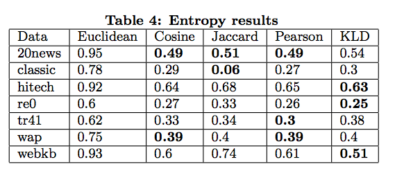
これを見ると、cos類似度もジャッカード類似度(から作った距離関数)も良い結果を出しています。
別にピアソン相関係数にこだわる必要はありません。いい結果なら試してみればいいのです。
この2つはscipyのcdistに距離関数として実装された上で用意されているので、パラメタを書くだけで、すぐに使えます。
cos距離
def new_euclidean_distances(X, Y=None, Y_norm_squared=None, squared=False):
    return cdist(X, Y, 'cosine')
ジャッカード距離
def new_euclidean_distances(X, Y=None, Y_norm_squared=None, squared=False):
    return cdist(X, Y, 'jaccard')
計測してみた
測ってみたのは、あくまで処理時間だけです。クラスタリング精度に関してはラベル付きデータを使っていないので、チェックしてません。
(今回の目的は、あくまで「論文で示された手法を使ってみたい」というモチベーションなので)
データは前回の記事と同じです。では順番にみていきましょう。
まずはノーマルのユークリッド距離です。数値はクラスタリングラベルと実行時間です。
[1 1 0 1 1 2 1 1 2 1 1 1 2 1 1 0 2 1 0 0 2 0 2 0 1 1 1 0 2 2 2 2 2 2 0 2 2]
Normal k-means:0.00853204727173
========================================
cos距離
[2 2 0 2 2 1 2 2 1 0 2 2 1 0 2 0 1 2 0 0 1 0 1 0 2 2 2 0 1 0 1 1 1 1 0 1 1]
Cosine k-means:0.0154190063477
========================================
ジャッカード距離
[0 0 0 0 1 0 0 0 2 0 0 0 1 0 0 0 0 0 2 2 0 2 0 2 0 0 0 0 2 2 0 0 0 0 0 0 0]
jaccard k-means:0.0656130313873
cdistを使ったピアソン相関係数
[0 0 0 1 1 2 1 0 2 1 0 2 2 0 0 1 1 0 1 0 2 0 2 0 2 2 1 1 2 1 1 2 2 2 1 2 2]
Special Coeficient k-means:9.39525008202
========================================
cython化したピアソン相関係数
[0 0 0 1 1 2 1 0 2 1 0 2 2 0 0 1 1 0 1 0 2 0 2 0 2 2 1 1 2 1 1 2 2 2 1 2 2]
Pearsonr k-means:9.40655493736
========================================
明らかにピアソン相関係数の実行時間は使い物になりません。速度は
ユークリッド < ジャッカード < cos < (越えられない壁) < ピアソン
でした。
ジャッカード係数距離はかなり結果がクラスタリングラベルがほかと違いますね・・・
もしかすると、今回は入力データが特徴量が小さい(文書クラスタリングとは大きく違う状況)なので、ほかと大きく違う結果になったのかもしれません。
このあたり、別の機会でしっかり検証していきたいと思います。
まとめ
scikit-learnのk-meansでほかの距離関数を使うには、
- cos類似度距離とジャッカード類似度距離はかなり実用的
- ピアソン相関係数はどうにもならぬ