これまでPytorch/Chainerメインで開発をしていたが、Tensorflow 2.0はデフォルトでDefine-By-Runをサポートしいるため、この機会に試してみた。
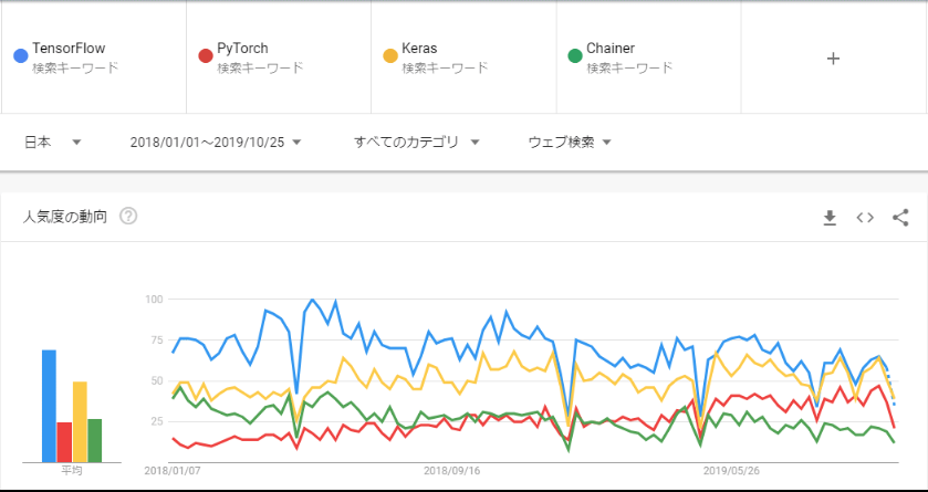
Googleトレンドでの比較で見てわかる通り、2018年後半からPytorchの人気がかなり上昇している。
TF2.0がEager Execution Mode(Define-By-Run)をデフォルトでサポートした真意は不明だが、少なからずPytorchの追い上げに関連してそう...
今更ではあるが、、
Caffe/TheanoのようなDefine-and-Runは、モデルをコンパイル(静的グラフ)を構築した後に、データを流し込む。それに対して、Pytorch/Chainerに代表されるDefine-By-Runはデータを流し込むタイミングで動的に計算グラフを構築する。
Define-by-Runのメリットとしては、入力データ構造に対して柔軟に対応が可能であり、コードのデバッグが容易であるが、最適化が困難というデメリットがある。対して、Define-and-Runのメリットは、最適化が容易である反面、データ構造の変化に対応しづらいというデメリットがある。
Define-by-Runについて、ある程度理解した上で、以下実際にコードに落とし込んでみる。
開発環境は画像データということもありローカルではさすがに時間が掛かるため、無料でGPU環境を提供しているGoogle Laboratryを使うことにした。
データは、Kaggleの以下データを使用
Chest X-Ray Images (Pneumonia):
https://www.kaggle.com/paultimothymooney/chest-xray-pneumonia
①Google Driveに配置したデータを取得するために必要なライブラリをインポート
from pydrive.auth import GoogleAuth
from pydrive.drive import GoogleDrive
from google.colab import auth
from oauth2client.client import GoogleCredentials
import os
②OAuth認証実行
auth.authenticate_user()
gauth = GoogleAuth()
gauth.credentials = GoogleCredentials.get_application_default()
drive = GoogleDrive(gauth)
③Google Driveデータダウンロード
def download_drive_data(save_folder, drive_folder_id):
  max_results = 100
  if not os.path.exists(save_folder):
      os.makedirs(save_folder)

  query = "'{}' in parents and trashed=false".format(drive_folder_id)

  for file_list in drive.ListFile({'q': query, 'maxResults': max_results}):
      for file in file_list:
          if file['mimeType'] == 'application/vnd.google-apps.folder':
              download_drive_data(os.path.join(save_folder, file['title']), file['id'])
          else:
              file.GetContentFile(os.path.join(save_folder, file['title']))

download_drive_data(save_folder='*****', drive_folder_id="*****")
③Tensorflow(GPU版)をインストール
!pip install tensorflow-gpu==2.0.0-rc1
④必要ライブラリのインポート
import numpy as np
%tensorflow_version 2.x
import tensorflow as tf
import cv2
import os
from sklearn.model_selection import train_test_split
from tensorflow.keras.layers import Dense, MaxPool2D, Dropout, BatchNormalization, InputLayer, GlobalAveragePooling2D, SeparableConv2D
from tensorflow.keras import Model
⑤バージョン確認
print(tf.__version__)
print(np.__version__)
print(cv2.__version__)

2.0.0
1.17.4
3.4.3
⑥GPUの使用するメモリ量を制限
physical_devices = tf.config.experimental.list_physical_devices('GPU')
assert len(physical_devices) > 0, "Not enough GPU hardware devices available"
tf.config.experimental.set_memory_growth(physical_devices[0], True)
⑥前処理用クラス
今回使用する画像は、サイズが統一されていないため、統一したサイズにリサイズする。また、トレーニング用データを増やすため、30度ずつ画像をローテートしAugmentationを実行している。画像サイズに関しては、Google Colabのメモリ上限の都合上少し小さめにしている。
class PreProcess:
  def __init__(self):
    self.height = 64
    self.width = 64
    self.angle = 30
    self.scale = 1.0
    self.aug_cnt = 5
    self.label_name_list = ['NORMAL', 'PNEUMONIA']

  #画像リサイズ処理
  def p_ps_img(self, file_path):
    for i, label_name in enumerate(self.label_name_list):
        if os.path.exists(file_path + str(i)) == False:
            os.mkdir(file_path + str(i))
            print(file_path + str(i) + ' has been created.')
        files = os.listdir(file_path + label_name)
        for file in files:
            img = cv2.imread(file_path + label_name + '/' + file)
            risize_img = cv2.resize(img, dsize=(self.height, self.width))
            grayed_img = cv2.cvtColor(risize_img, cv2.COLOR_BGR2GRAY)
            if 'train' in file_path:
              int_angle = 0
              for rotate_num in range(self.aug_cnt):
                int_angle += self.angle
                augmated_img = self.__aug_img(grayed_img, int_angle)
                cv2.imwrite(file_path + str(i) + '/' + file + '_' + str(rotate_num) + '.jpg', augmated_img)
            else:
              cv2.imwrite(file_path + str(i) + '/' + file, grayed_img)

  #画像データ読み込み
  def load_data(self, file_path):
    img_list = []
    y_list = []
    for label in range(2):
        files = os.listdir(file_path + str(label))
        for file in files:
            img = cv2.imread(file_path + str(label) + '/' + file)
            img_list.append(img)
            y_list.append(label)

    return img_list, y_list

  #ローテート処理
  def __aug_img(self, img, int_angle):
    size = (self.height, self.width)
    center = (int(size[0]/2), int(size[1]/2))
    angle = int_angle
    scale = self.scale
    rotation_matrix = cv2.getRotationMatrix2D(center, angle, scale)
    rotated = cv2.warpAffine(img, rotation_matrix, size)

    return rotated
⑦前処理実行
train_path = '/content/chest_xray/train/'
test_path = '/content/chest_xray/test/'
pre_ps = PreProcess()
pre_ps.p_ps_img(train_path)
pre_ps.p_ps_img(test_path)
実際の前処理後の画像は以下のようになる。

⑧学習/テスト用データをロード
X_train_list, y_train_list = pre_ps.load_data(train_path)
X_test_list, y_test_list = pre_ps.load_data(test_path)
⑨Numpy配列に変換
X_train, y_train, X_test, y_test = np.array(X_train_list), np.array(y_train_list), np.array(X_test_list), np.array(y_test_list)
⑩入力データの正規化
X_train, X_test = X_train / 255.0, X_test / 255.0
⑪ミニバッチ作成
train_ds = tf.data.Dataset.from_tensor_slices(
    (X_train, y_train)).shuffle(X_train.shape[0]).batch(64)
test_ds = tf.data.Dataset.from_tensor_slices(
    (X_test, y_test)).shuffle(X_test.shape[0]).batch(64)
⑫ネットワーク層(CNN)
オブジェクト指向型な記載方法をサポートしており、Pytorch/Chainerに慣れている人にとってはとっつきやすい。
tensorflow.keras.Modelを継承しており、Pytorchで言えばnn.Moduleに該当する。
データを入力したタイミングでcallメソッドが呼び出される。
class cnnModel(Model):
  def __init__(self, width, height, channel, batch_size, output_dim):
    super(cnnModel, self).__init__()
    self.inlayer = InputLayer(input_shape=(width, height, channel), batch_size=batch_size)
    self.sconv1 = SeparableConv2D(32, 3, activation='relu')
    self.sconv2 = SeparableConv2D(64, 3, activation='relu')
    self.pool1 = MaxPool2D(pool_size=(2, 2))
    self.btnorm1 = BatchNormalization()
    self.do1 = Dropout(0.5)
    self.sconv3 = SeparableConv2D(128, 3, activation='relu')
    self.sconv4 = SeparableConv2D(256, 3, activation='relu')
    self.pool2 = MaxPool2D(pool_size=(2, 2))
    self.btnorm2 = BatchNormalization()
    self.do2 = Dropout(0.5)
    self.sconv5 = SeparableConv2D(512, 3, activation='relu')
    self.sconv6 = SeparableConv2D(512, 3, activation='relu')
    self.pool3 = MaxPool2D(pool_size=(2, 2))
    self.btnorm3 = BatchNormalization()
    self.do3 = Dropout(0.5)
    self.gapool1 = GlobalAveragePooling2D()
    self.d1 = Dense(1024, activation='relu')
    self.do4 = Dropout(0.5)
    self.d2 = Dense(64, activation='relu')
    self.do5 = Dropout(0.5)
    self.d3 = Dense(output_dim, activation='softmax')

  def call(self, x):
    x = self.inlayer(x)
    x = self.sconv1(x)
    x = self.sconv2(x)
    x = self.pool1(x)
    x = self.btnorm1(x)
    x = self.do1(x)
    x = self.sconv3(x)
    x = self.sconv4(x)
    x = self.pool2(x)
    x = self.btnorm2(x)
    x = self.do2(x)
    x = self.sconv5(x)
    x = self.sconv6(x)
    x = self.pool3(x)
    x = self.btnorm3(x)
    x = self.do3(x)
    x = self.gapool1(x)
    x = self.d1(x)
    x = self.do4(x)
    x = self.d2(x)
    x = self.do5(x)

    return self.d3(x)
⑬学習/予測/評価クラス
デフォルトでは、Eager Executionとして実行されるが、バッチごとに計算グラフを構築するため、パフォーマンス観点からは、あまり好ましくない。そのため、学習/予測実行関数に対しては、アノテーションに@tf.functionを付与し、Graph Modeで実行(静的グラフにコンパイル)することでパフォーマンス上の問題を改善できる。
また、エポック毎にチェックポイントを生成し、次回学習時に前回学習終了時点のパラメータを復元できるようにした。
TFのチェックポイントの仕組みとしては、変数をロードされたオブジェクトから始めて、名前付けられたエッジ(オブジェクトの属性)を持つ有向グラフを辿ることによりチェックポイントされた値に合わせる。
tf.train.Checkpoint オブジェクト上の restore() 呼び出しは要求された復元をキューに入れて、Checkpoint オブジェクトから一致するパスがあった場合に変数値を復元する。つまり、定義したモデルから単にカーネルをネットワークと層を通してそれへのパスを再構築することによりパラメータを復元する。

class Trainer:
  def __init__(self, model):
    self.model = model

    #誤差/最適化関数
    lr = 1e-4
    self.loss_object = tf.keras.losses.SparseCategoricalCrossentropy()
    self.optimizer = tf.keras.optimizers.Adam(learning_rate=lr)

    #評価関数
    self.train_loss = tf.keras.metrics.Mean(name='train_loss')
    self.train_accuracy = tf.keras.metrics.SparseCategoricalAccuracy(name='train_accuracy')
    self.test_loss = tf.keras.metrics.Mean(name='test_loss')
    self.test_accuracy = tf.keras.metrics.SparseCategoricalAccuracy(name='test_accuracy')

    max_keep = 10
    self.chk_point_path = './tf_ckpts'
    self.ckpt = tf.train.Checkpoint(step=tf.Variable(1), optimizer=self.optimizer, model=self.model)
    self.manager = tf.train.CheckpointManager(self.ckpt, self.chk_point_path, max_to_keep=max_keep)

  #学習実行関数(グラフモード)
  @tf.function
  def train_step(self, image, label):
    with tf.GradientTape() as tape:
      predictions = self.model(image)
      loss = self.loss_object(label, predictions)

    gradients = tape.gradient(loss, self.model.trainable_variables)
    self.optimizer.apply_gradients(zip(gradients, self.model.trainable_variables))

    self.train_loss(loss)
    self.train_accuracy(label, predictions)

  #検証実行関数(グラフモード)
  @tf.function
  def test_step(self, image, label):
    predictions = self.model(image)
    t_loss = self.loss_object(label, predictions)

    self.test_loss(t_loss)
    self.test_accuracy(label, predictions)

  #学習/予測/評価実行
  def train_test_fn(self, epochs, train_ds, test_ds):
    #既存チェックポイントからのリストア
    self.ckpt.restore(self.manager.latest_checkpoint)
    if self.manager.latest_checkpoint:
      print("チェックポイント {} をリストア...".format(self.manager.latest_checkpoint))
    else:
      print("チェックポイントが存在しないため、初期状態からの学習...")

    for epoch in range(epochs):
      for image, label in train_ds:
        with tf.device("/gpu:0"):
          self.train_step(image, label)

      for test_image, test_label in test_ds:
        with tf.device("/gpu:0"):
          self.test_step(test_image, test_label)

      if (epoch + 1) % 1 == 0:
        template = 'Epoch {}, Loss: {:.5f}, Accuracy: {:.5f}, Test Loss: {:.5f}, Test Accuracy: {:.5f}'
        print (template.format(epoch+1,
                              self.train_loss.result(),
                              self.train_accuracy.result()*100,
                              self.test_loss.result(),
                              self.test_accuracy.result()*100))

      #エポック毎にチェックポイント保存
      self.ckpt.step.assign_add(1)
      if int(self.ckpt.step) % 1 == 0:
        save_path = self.manager.save()
        print("チェックポイントを保存: {}".format(int(self.ckpt.step), save_path))
⑭モデルの初期化
cnn_model = cnnModel(X_train.shape[1], X_train.shape[2], X_train.shape[3], batch_size=32, output_dim=2)
⑮学習/評価
trainer = Trainer(cnn_model)
trainer.train_test_fn(epochs=50, train_ds=train_ds, test_ds=test_ds)

チェックポイントが存在しないため、初期状態からの学習...
Epoch 1, Loss: 0.57603, Accuracy: 74.23697, Test Loss: 0.68871, Test Accuracy: 62.50000
チェックポイントを保存: 2
Epoch 2, Loss: 0.56901, Accuracy: 74.33090, Test Loss: 0.58955, Test Accuracy: 71.07372
チェックポイントを保存: 3
Epoch 3, Loss: 0.49160, Accuracy: 77.48338, Test Loss: 0.52456, Test Accuracy: 74.89317
チェックポイントを保存: 4
Epoch 4, Loss: 0.44060, Accuracy: 79.77665, Test Loss: 0.50206, Test Accuracy: 75.88141
チェックポイントを保存: 5
Epoch 5, Loss: 0.40814, Accuracy: 81.32285, Test Loss: 0.48017, Test Accuracy: 77.11539
チェックポイントを保存: 6
Epoch 6, Loss: 0.38605, Accuracy: 82.38369, Test Loss: 0.46281, Test Accuracy: 78.15171
チェックポイントを保存: 7
Epoch 7, Loss: 0.36836, Accuracy: 83.27782, Test Loss: 0.45715, Test Accuracy: 78.22802
チェックポイントを保存: 8
⑯学習再開
チェックポイント ./tf_ckpts/ckpt-8 をリストア...
Epoch 1, Loss: 0.34058, Accuracy: 84.69032, Test Loss: 0.44556, Test Accuracy: 78.82835
・
・
Epoch 19, Loss: 0.22930, Accuracy: 90.27736, Test Loss: 0.41090, Test Accuracy: 82.16999
チェックポイントを保存: 28
Epoch 20, Loss: 0.22587, Accuracy: 90.44373, Test Loss: 0.41324, Test Accuracy: 82.21153
チェックポイントを保存: 29
Epoch 21, Loss: 0.22260, Accuracy: 90.60131, Test Loss: 0.41246, Test Accuracy: 82.33311
チェックポイントを保存: 30
Epoch 22, Loss: 0.21943, Accuracy: 90.75378, Test Loss: 0.41382, Test Accuracy: 82.39851
チェックポイントを保存: 31
Epoch 23, Loss: 0.21633, Accuracy: 90.90470, Test Loss: 0.41248, Test Accuracy: 82.48553
チェックポイントを保存: 32
Epoch 24, Loss: 0.21344, Accuracy: 91.04456, Test Loss: 0.41313, Test Accuracy: 82.50200
チェックポイントを保存: 33
Epoch 25, Loss: 0.21065, Accuracy: 91.17853, Test Loss: 0.41447, Test Accuracy: 82.52720