Tensorflow チュートリアルのStyle Transferを読み解く

1. はじめに

Style Transfer(スタイルトランスファー)の例を見て、自分でも試してみたいと思い、
TensorFlowのチュートリアルにあるコードを実行してみました。

初学者の私には色々と調べなければわからない部分もあり、
備忘録としてまとめさせていただきます。

2. Style Tranferとは

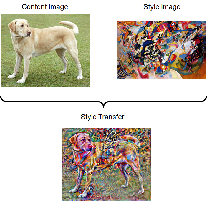
Style Transferとは、ある画像に対して、他の画像の特徴(絵で言えば”作風")を反映し、
もとの画像からスタイルを変更させることです。

チュートリアルでは犬の画像に対して、ワシリー・カンディンスキーの絵の特徴を取り入れることで、
"もしその画像をワシリー・カンディンスキーが描いたら？"を想像させるような、
画像の生成を行っています。

3. コード確認

3-1. 設定

まずは必要なモジュールをインポートしています。
mpl.rcParamsはグラフの共通の初期設定を行っています。

import os
import tensorflow as tf
# Load compressed models from tensorflow_hub
os.environ['TFHUB_MODEL_LOAD_FORMAT'] = 'COMPRESSED'

import IPython.display as display

import matplotlib.pyplot as plt
import matplotlib as mpl
mpl.rcParams['figure.figsize'] = (12, 12)
mpl.rcParams['axes.grid'] = False

import numpy as np
import PIL.Image
import time
import functools

次にテンソルをPIL.Imageに変換する関数を定義しています。
これは学習が進行するごとに、画像がどう変化していくかを見る際に使用します。

def tensor_to_image(tensor):
  tensor = tensor*255
  tensor = np.array(tensor, dtype=np.uint8)
  if np.ndim(tensor)>3:
    assert tensor.shape[0] == 1
    tensor = tensor[0]
  return PIL.Image.fromarray(tensor)

次に画像を参照URLからダウンロードし保存します。
tf.keras.utils.get_fileはURL先のデータがキャッシュになければダウンロードを行い、
その保存された先のパスを返します。
(パスの例：C:\Users\{USERNAME}\.keras\datasets\YellowLabradorLooking_new.jpg)

content_path = tf.keras.utils.get_file('YellowLabradorLooking_new.jpg', 'https://storage.googleapis.com/download.tensorflow.org/example_images/YellowLabradorLooking_new.jpg')
style_path = tf.keras.utils.get_file('kandinsky5.jpg','https://storage.googleapis.com/download.tensorflow.org/example_images/Vassily_Kandinsky%2C_1913_-_Composition_7.jpg')

3-2. 入力を視覚化する

画像を読み込み、最大サイズを512ピクセル(max_dim)にします。
max_dimと実際の画像の最大サイズ(long_dim)の比をとり(scale)、
もう一方の辺にも適用しています。

def load_img(path_to_img):
  max_dim = 512
  img = tf.io.read_file(path_to_img)
  img = tf.image.decode_image(img, channels=3)
  img = tf.image.convert_image_dtype(img, tf.float32)

  shape = tf.cast(tf.shape(img)[:-1], tf.float32)
  long_dim = max(shape)
  scale = max_dim / long_dim

  new_shape = tf.cast(shape * scale, tf.int32)

  img = tf.image.resize(img, new_shape)
  img = img[tf.newaxis, :]
  return img

content_image = load_img(content_path)
style_image = load_img(style_path)

上記コードのcontent_imageがStyle Transferを適用する前の元画像。
style_imageが作風を取り入れる参考画像(スタイル画像)となります。

3-3. コンテンツとスタイルの表現を定義する

今回は実際の実行には直接関係しない部分は適宜飛ばして進めていきます。
このチュートリアルではVGG19のimagenetについて学習したモデルを引用しています。
まず下記コードでVGG19のレイヤー一覧を出力します。

vgg = tf.keras.applications.VGG19(include_top=False, weights='imagenet')

print()
for layer in vgg.layers:
  print(layer.name)

結果

input_2
block1_conv1
block1_pool
・・・
block5_conv4
block5_pool

そのうち、Contents Lossの計算に用いる層と
Style Lossの計算に用いる層を定義します。

Contents Lossは元画像(content_image)を維持するための誤差で、
更新中の画像と元画像のある層での出力の2乗誤差で定義します。
更新中の画像と元の画像の特徴が近ければ、
ある層での出力も近いだろうという考え方です。

Style Lossはスタイルを適用するための誤差で、
更新中の画像とスタイル画像(style_image)のある層での出力の
グラム行列計算結果の2乗誤差で定義します。
更新中の画像とスタイル画像の特徴が近ければ、
ある層での出力のグラム行列計算結果も近いだろうという考え方です。

content_layers = ['block5_conv2'] 

style_layers = ['block1_conv1',
                'block2_conv1',
                'block3_conv1', 
                'block4_conv1', 
                'block5_conv1']

num_content_layers = len(content_layers)
num_style_layers = len(style_layers)

中間層から抜き取ることについては、以下のような説明が記載されています。

Intermediate layers for style and content
スタイルとコンテンツのための中間層

So why do these intermediate outputs within our pretrained image classification network allow us to define style and content representations?
なぜ画像認識のために学習されたネットワークの中間層出力がスタイルとコンテンツを表現するのに役立つのでしょうか？

At a high level, in order for a network to perform image classification (which this network has been trained to do), it must understand the image. This requires taking the raw image as input pixels and building an internal representation that converts the raw image pixels into a complex understanding of the features present within the image.
高次では学習が行われたネットワークが画像認識をするためには、画像を理解する必要があります。
そのためには、入力される生の画像データを複雑な理解ができるような特徴に変換するような、
内部表現が必要となります。

This is also a reason why convolutional neural networks are able to generalize well: they’re able to capture the invariances and defining features within classes (e.g. cats vs. dogs) that are agnostic to background noise and other nuisances. Thus, somewhere between where the raw image is fed into the model and the output classification label, the model serves as a complex feature extractor. By accessing intermediate layers of the model, you're able to describe the content and style of input images.
これは畳み込みニューラルネットワークがなぜ汎化性が高いかの理由にもなります。
これらのネットワークは画像を不変的に形づくる特徴を読み取り、クラスに分けることができ、
バックグラウンドノイズやその他の余計なものは認識しません。
つまり、入力される生の画像データと出力されるクラス分類の間で、モデルは複雑な特徴量抽出を行っています。
その中間層にアクセスすることにより、コンテンツやスタイルの画像をうまく表現することができます。

3-4. モデルを構築する

中間層の名前(layer_names)をあたえることで、
その層での出力を返すモデルを作成します。

今回は画像の各ピクセルの値を最適化手法により変更し、ネットワークの結合係数は変更しないことから、
vgg.trainable = Falseとします。

def vgg_layers(layer_names):
  """ Creates a vgg model that returns a list of intermediate output values."""
  # Load our model. Load pretrained VGG, trained on imagenet data
  vgg = tf.keras.applications.VGG19(include_top=False, weights='imagenet')
  vgg.trainable = False

  outputs = [vgg.get_layer(name).output for name in layer_names]

  model = tf.keras.Model([vgg.input], outputs)
  return model

3-5. スタイルを計算する

ある中間層でのスタイルの出力のグラム行列計算は以下の数式に基づいています。

G_{cd}^l = \frac {\sum_{ij} F_{ijc}^l(x) F_{ijd}^l(x)}{IJ}

def gram_matrix(input_tensor):
  result = tf.linalg.einsum('bijc,bijd->bcd', input_tensor, input_tensor)
  input_shape = tf.shape(input_tensor)
  num_locations = tf.cast(input_shape[1]*input_shape[2], tf.float32)
  return result/(num_locations)

einsumによって簡潔に計算できますと書いてありますが、
einsumとは下記数式のごとく計算を行ってくれる関数のようです。

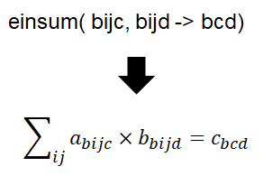
ここの計算が自分のなかでよく理解できなかったので、
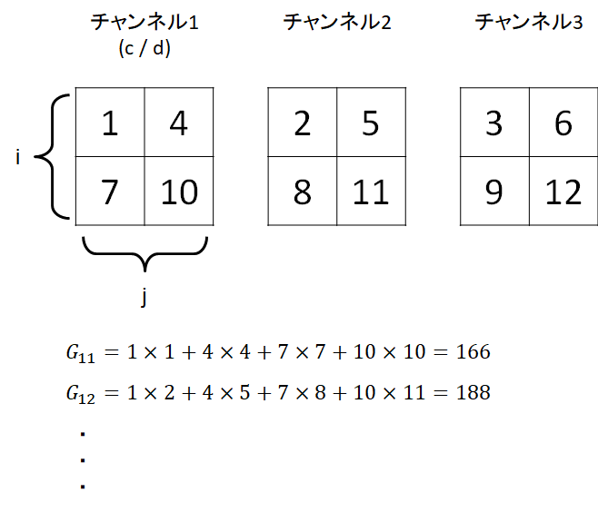
簡単な数字を入れて試してみました。

a = [[ [[1,2,3],[4,5,6]] , [[7,8,9],[10,11,12]] ]]
t_a = tf.convert_to_tensor(a)

print(gram_matrix(t_a))

結果

tf.Tensor(
[[[166 188 210]
  [188 214 240]
  [210 240 270]]], shape=(1, 3, 3), dtype=int32)

イメージこのような感じだと思います。
間違っていたらご指摘もらえると幸いです。

3-6. スタイルとコンテンツを抽出する

スタイルとコンテンツを返すクラスを作成します。

class StyleContentModel(tf.keras.models.Model):
  def __init__(self, style_layers, content_layers):
    super(StyleContentModel, self).__init__()
    self.vgg = vgg_layers(style_layers + content_layers)
    self.style_layers = style_layers
    self.content_layers = content_layers
    self.num_style_layers = len(style_layers)
    self.vgg.trainable = False

  def call(self, inputs):
    "Expects float input in [0,1]"
    inputs = inputs*255.0
    preprocessed_input = tf.keras.applications.vgg19.preprocess_input(inputs)
    outputs = self.vgg(preprocessed_input)
    style_outputs, content_outputs = (outputs[:self.num_style_layers],
                                      outputs[self.num_style_layers:])

    #style_outputsにはグラム行列を適用
    style_outputs = [gram_matrix(style_output)
                     for style_output in style_outputs]

    content_dict = {content_name: value
                    for content_name, value
                    in zip(self.content_layers, content_outputs)}

    style_dict = {style_name: value
                  for style_name, value
                  in zip(self.style_layers, style_outputs)}

    return {'content': content_dict, 'style': style_dict}

#オブジェクトの作成
extractor = StyleContentModel(style_layers, content_layers)

3-7. 最急降下法を実行します

まずスタイルとコンテンツのターゲット値を設定します。
style_targetsにはスタイル画像(style_image)を入力し、
content_targetには元画像(content_image)を入力します。

style_targets = extractor(style_image)['style']
content_targets = extractor(content_image)['content']

content_imageは変数として設定します。

image = tf.Variable(content_image)

フロート画像なので、0から1に収めるようにします。

def clip_0_1(image):
  return tf.clip_by_value(image, clip_value_min=0.0, clip_value_max=1.0)

オプティマイザはAdamにしています。
(論文ではLBFGSを推奨しているようです。)

opt = tf.optimizers.Adam(learning_rate=0.02, beta_1=0.99, epsilon=1e-1)

style_weight=1e-2
content_weight=1e4

損失の計算を行う関数を定義します。
style_output/content_outputは更新中の画像での各層での出力、
style_targetsはスタイル画像の各層での出力、
content_targetsは元画像の各層での出力となります。

style_lossは更新中の画像の出力とスタイル画像の出力のグラム行列の2乗誤差をとり、
使用した層数で割って正規化しています。

content_lossは更新中の画像の出力と元画像の出力の2乗誤差をとり、
使用した層数で割って正規化しています。

最後に各Lossの加重平均をとります。

def style_content_loss(outputs):
    style_outputs = outputs['style']
    content_outputs = outputs['content']
    style_loss = tf.add_n([tf.reduce_mean((style_outputs[name]-style_targets[name])**2) 
                           for name in style_outputs.keys()])
    style_loss *= style_weight / num_style_layers

    content_loss = tf.add_n([tf.reduce_mean((content_outputs[name]-content_targets[name])**2) 
                             for name in content_outputs.keys()])
    content_loss *= content_weight / num_content_layers
    loss = style_loss + content_loss
    return loss

3-8. 全変動損失

この基本的な構成の1つの欠点は、人工的な高周波のノイズを生成してしまう点です。
これは正則化項を入れることで減らすことができ、Style Tranferでは、全変動損失(Total variation loss)と呼ばれることが一般的です。

これはとなりのピクセルとの差をとり、その絶対値の総和をとることで計算でき、
各ピクセルをなめらかにつなぐ効果があります。

関数を定義すると以下の通りです。

def high_pass_x_y(image):
  x_var = image[:, :, 1:, :] - image[:, :, :-1, :]
  y_var = image[:, 1:, :, :] - image[:, :-1, :, :]

  return x_var, y_var

def total_variation_loss(image):
  x_deltas, y_deltas = high_pass_x_y(image)
  return tf.reduce_sum(tf.abs(x_deltas)) + tf.reduce_sum(tf.abs(y_deltas))

ですが、実際はtensorflowの以下の関数で計算できるため、
上記記述は不要とのことです。

tf.image.total_variation(image)

3-9. 最適化の実行

total_variation_lossのウェイトを定義し、
勾配計算を記述します。

total_variation_weight=30

@tf.function()
def train_step(image):
  with tf.GradientTape() as tape:
    outputs = extractor(image)
    loss = style_content_loss(outputs)
    loss += total_variation_weight*tf.image.total_variation(image)

  grad = tape.gradient(loss, image)
  opt.apply_gradients([(grad, image)])
  image.assign(clip_0_1(image))

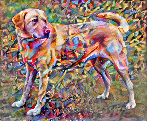
最適化計算を実行します。

import time
start = time.time()

epochs = 10
steps_per_epoch = 100

step = 0
for n in range(epochs):
  for m in range(steps_per_epoch):
    step += 1
    train_step(image)
    print(".", end='', flush=True)
  display.clear_output(wait=True)
  display.display(tensor_to_image(image))
  print("Train step: {}".format(step))

end = time.time()
print("Total time: {:.1f}".format(end-start))

結果

4.　まとめ

今回はTensor flowのチュートリアルStyle Tranferに沿って勉強をしてみました。
細かいところを調べながらでき、少しは身になったかと思います。