1. 背景
前回はCelebAの画像をローカルに落とし、そこからtensorflow_datasets形式にするまでをまとめました。
今回はそれらのデータセットから、性別判定をするソフトを畳み込みニューラルネットワーク(CNN)によって作成しようと思います。
2. 方法
2-1. データの前処理
まず、データセットを訓練データ(10000) / 検証データ(1000) / テストデータ(1000) に切り分けます。
reshuffle_each_iterationをFalseにしておくことで、それぞれのデータを切り分けるときに、
毎回同じ順番でシャッフルされ、ある画像が訓練データとテストデータ両方に混ざりこむようなことを避けてくれます。
tf.random.set_seed(1)
ds_images_labels = ds_images_labels.shuffle(1000,reshuffle_each_iteration=False)
celeba_train = ds_images_labels.take(10000)
celeba_valid = ds_images_labels.skip(10000).take(1000)
celeba_test = ds_images_labels.skip(11000).take(1000)
次にデータ拡張(データの水増し)を行います。データ拡張とは、元データに対して(ランダム的に)加工を入れることによって、少ないデータセットでも過学習を抑制し、汎化性を向上させるものだと認識しています。
def preprocess(example_i,example_l,size=(64,64),mode='train'):
    """訓練時:画像をランダムに変形、テスト時:画像を整形して返す関数"""
    image = example_i
    label = example_l[20]  #ラベル21列目が性別

    if mode == 'train':
        image_cropped = tf.image.random_crop(image,size=(150,150,3))
        image_resized = tf.image.resize(image_cropped,size = size)
        image_flip = tf.image.random_flip_left_right(image_resized)
        return (image_flip, tf.cast(label,tf.int32))
    else:
        image_cropped = tf.image.crop_to_bounding_box(
            image,offset_height=34,offset_width=14,
            target_height=150,target_width=150)
        image_resized = tf.image.resize(image_cropped,size=size)
        return (image_resized, tf.cast(label,tf.int32))
tf.image.random_cropがランダムに画像を切り取る関数(訓練時に使用)。
tf.image.crop_to_bounding_boxが毎回決まった位置で画像を切り取る関数(テスト時に使用)です。
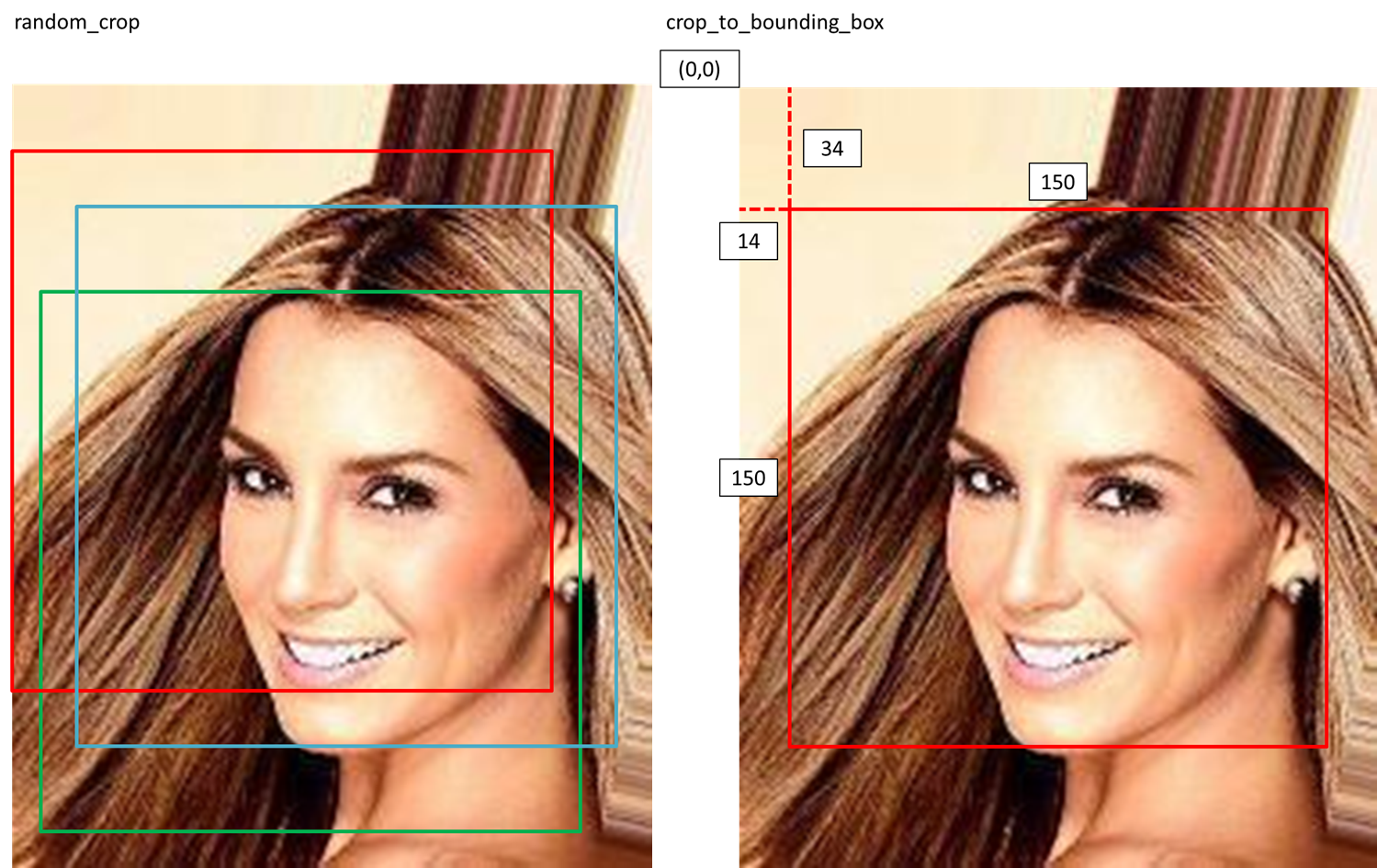
tf.image.resizeは画像のサイズを変える関数、
tf.image.random_flip_left_rightはランダムに画像を左右反転する関数です。
次に上記の関数をデータセットに適用します。
BATCH_SIZE = 32
BUFFER_SIZE = 1000
IMAGE_SIZE = (64,64)
steps_per_epoch = np.ceil(16000/BATCH_SIZE) #画像数/バッチ数
# dsが(img, label)のタプルのため、lambdaに二つ引数を渡す。
ds_train = celeba_train.map(lambda x,i:preprocess(x,i,size=(178,178),mode='train'))
ds_train = ds_train.shuffle(buffer_size=BUFFER_SIZE).repeat()
ds_train = ds_train.batch(BATCH_SIZE)

ds_valid = celeba_valid.map(lambda x,i:preprocess(x,i,size=(178,178),mode='train'))
ds_valid = ds_valid.batch(BATCH_SIZE)
これでデータの前処理は完了です。
2-2. 学習
CNNを構築し、学習を行います。
ネットワークの概要は以下の通りです。
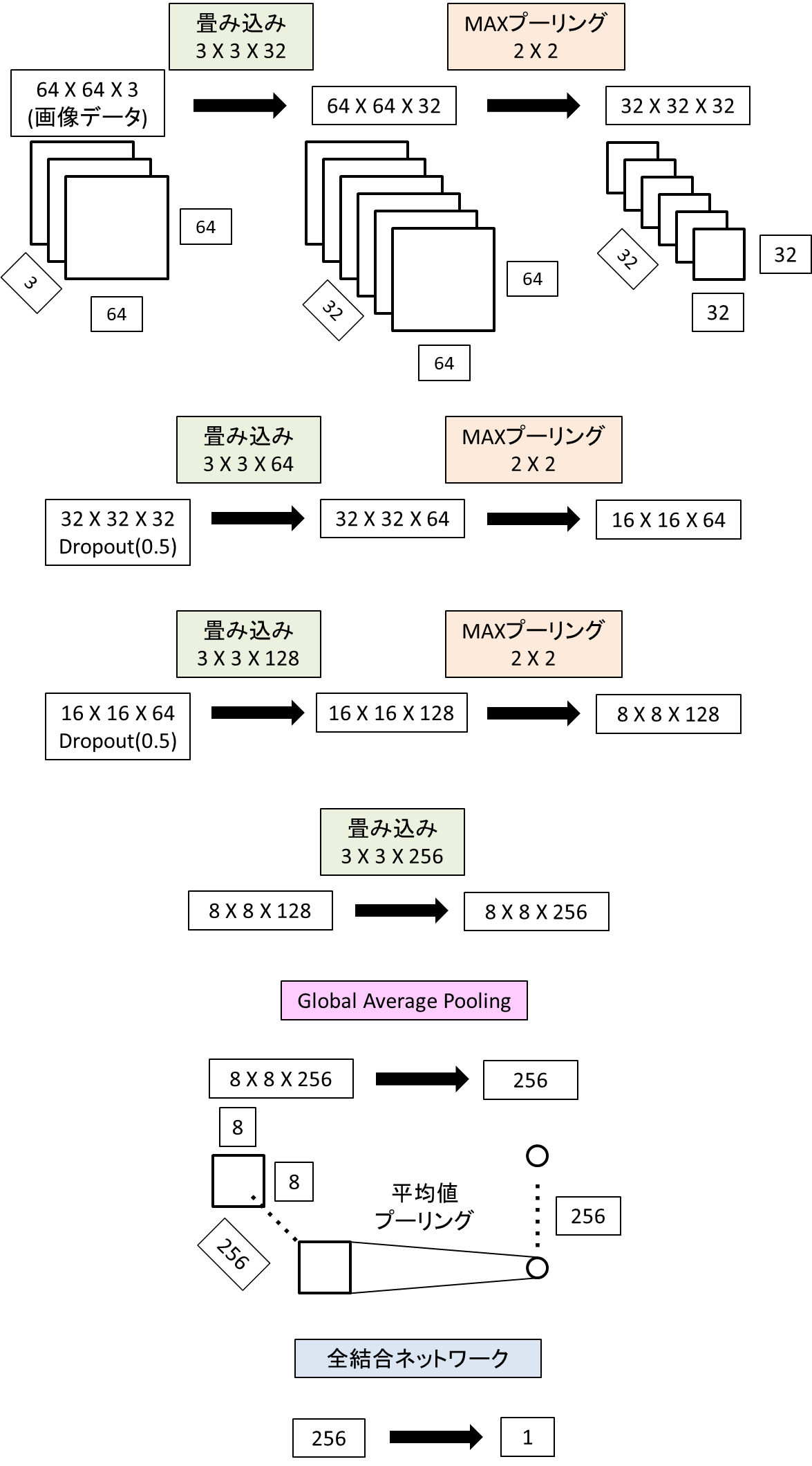
model = tf.keras.Sequential([
    tf.keras.layers.Conv2D(32,(3,3),padding='same',activation='relu'),
    tf.keras.layers.MaxPooling2D((2,2)),
    tf.keras.layers.Dropout(rate=0.5),

    tf.keras.layers.Conv2D(64,(3,3),padding='same',activation='relu'),
    tf.keras.layers.MaxPooling2D((2,2)),
    tf.keras.layers.Dropout(rate=0.5),

    tf.keras.layers.Conv2D(128,(3,3),padding='same',activation='relu'),
    tf.keras.layers.MaxPooling2D((2,2)),

    tf.keras.layers.Conv2D(256,(3,3),padding='same',activation='relu'),

    #GlobalAveragePooling 8X8X256 -> 256
    tf.keras.layers.GlobalAveragePooling2D(),

    tf.keras.layers.Dense(1,activation=None)
    ])

model.compile(optimizer = tf.keras.optimizers.Adam(),
                loss=tf.keras.losses.BinaryCrossentropy(from_logits=True),
                metrics=['accuracy'])
history = model.fit(ds_train,validation_data=ds_valid,
                    epochs=20,steps_per_epoch=steps_per_epoch)
3. 結果
3-1. 損失関数と正解率
損失関数と正解率の変動をグラフ化する。
hist = history.history
x_arr = np.arange(len(hist['loss'])) + 1
fig = plt.figure(figsize=(12,4))
ax = fig.add_subplot(1,2,1)
ax.plot(x_arr, hist['loss'], '-o', label='Train loss')
ax.plot(x_arr, hist['val_loss'],'--<', label='Validation loss')
ax.legend(fontsize=15)
ax.set_xlabel('Epoch', size=15)
ax.set_ylabel('Loss', size=15)
ax = fig.add_subplot(1,2,2)
ax.plot(x_arr,hist['accuracy'],'-o',label='Train acc.')
ax.plot(x_arr,hist['val_accuracy'],'--<',label='Validation acc.')
ax.legend(fontsize=15)
ax.set_xlabel('Epoch',size=15)
ax.set_ylabel('accuracy',size=15)
plt.show()

Epochを経て損失関数の低下と正答率の増加が分かります。
次にテストデータでの正解率を計算します。
# テストデータ
ds_test = celeba_test.map(lambda x,i:preprocess(x,i,size=(64,64),mode='eval')).batch(32)
test_results = model.evaluate(ds_test,verbose=0)
print('Test Acc: {:.2f}%'.format(test_results[1]*100))
結果
Test Acc: 94.00%
正解率は94%となりました。
3-2. 判定された画像を表示
以下4つのパターンに分けて画像を表示します。
・正しく判定されたMale画像
・誤って判定されたMale画像
・正しく判定されたFemale画像
・誤って判定されたFemale画像
ds = ds_test.unbatch().take(100).batch(100)
pred_logits = model.predict(ds)
probas = tf.sigmoid(pred_logits)
# Maleの確率が0.5以上の画像はMale、それ以外はFemaleと判定
preds = [1 if x >= 0.5 else 0 for x in probas]
image_list = []
label_list = []
for i in ds:
    image_list.append(i[0].numpy())
    label_list.append(i[1].numpy())

image_list = np.array(image_list)
label_list = np.array(label_list)

# 正しく判定されたイメージリスト/ラベルリストと間違って判定されたイメージリスト/ラベルを作成
c_image = image_list[preds == label_list]
c_label = label_list[preds == label_list]
w_image = image_list[preds != label_list]
w_label = label_list[preds != label_list]
# 正しく判定されたmaleイメージリストとfemaleイメージリスト
m_c_image = c_image[[True if x == 1 else False for x in c_label]]
f_c_image = c_image[[False if x == 1 else True for x in c_label]]
# 誤って判定されたmaleイメージリストとfemaleイメージリスト
m_w_image = w_image[[True if x == 1 else False for x in w_label]]
f_w_image = w_image[[False if x == 1 else True for x in w_label]]

# matplotで画像を表示
fig = plt.figure(figsize=(6,10))
for j,example in enumerate(m_c_image[:3]):
     ax = fig.add_subplot(4,3,j+1)
     ax.set_xticks([]);ax.set_yticks([])
     ax.imshow(example)
     if j == 0:
        ax.set_title('Label:Male, Predict:Male',loc='left',pad=4,size=12)

for j,example in enumerate(m_w_image[:3]):
     ax = fig.add_subplot(4,3,j+4)
     ax.set_xticks([]);ax.set_yticks([])
     ax.imshow(example)
     if j == 0:
        ax.set_title('Label:Male, Predict:Female',loc='left',pad=4,size=12)

for j,example in enumerate(f_c_image[:3]):
     ax = fig.add_subplot(4,3,j+7)
     ax.set_xticks([]);ax.set_yticks([])
     ax.imshow(example)
     if j == 0:
        ax.set_title('Label:Female, Predict:Female',loc='left',pad=4,size=12)

for j,example in enumerate(f_w_image[:3]):
     ax = fig.add_subplot(4,3,j+10)
     ax.set_xticks([]);ax.set_yticks([])
     ax.imshow(example)
     if j == 0:
        ax.set_title('Label:Female, Predict:Male',loc='left',pad=4,size=12)

plt.show()
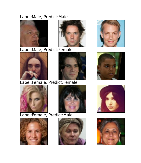
上の行から
・正しく判定されたMale画像
・誤って判定されたMale画像
・正しく判定されたFemale画像
・誤って判定されたFemale画像
になります。
あくまで個人的な感想ですが、髪の長さは判定に影響を与えていそうだなと思いました。
そう思った理由は以下の2つです。
・誤って判定されたMale画像の一番左は髪が長い。
・誤って判定されたFemale画像の右2つは写真上は髪があまり露出していない。
実際NNによる判定はブラックボックス化されているので、この感想の真偽を確かめるのは難しそうですが。。。
4. まとめ
CNNを用いてCelebAの画像の性別判定をしました。
誤った画像を見ると、人の判断では間違えなさそうですね。
シンプルなCNNを使ってみただけなので、性能はまだ上げられそうだなと思いました。