遅ればせながら,CourseraのMaechine Learning (Stanford University, by Andrew Ng)を受講している.もちろん説明動画も有益だが,このコースの良さを際立させているのが,毎回出されるプログラミングの課題である.ただMatlabのコードなので,後で復習できるようにPythonに書き換えたくなってきた.(他の方で,同じ取り組みの紹介例がInternetで見受けられる.)
ここでは,"Coursera / Machine Learning"の教材を(Pythonで)2度3度楽しむやり方を紹介する.また関数最小化で用いる,scipy.optimize.minimize() について説明する.
コスト関数とその導関数
Machine Learningの教材では,コスト関数を作成し,それを最小化するパラメータを探索する,というものが多い.Matlabでは fminunc() (あるいは課題で用意されていたfmincg() )を使うのだが,Pythonでは同様の機能を**scipy.optimize.minimize()**がサポートしている.
まず,コスト関数とその導関数を自前で用意する.第一回の課題,線形モデルでは次の式で与えられる.
J(\theta) = \frac{1}{2m} \sum_{i=1}^{m} (h_{\theta}(x ^{(i)} ) -y ^{(i)}) ^2
\\
\frac{\partial J}{\partial \theta _j} = \frac{1}{m} \sum_{i=1}^{m}
(h_{\theta} (x^{(i)}) - y^{(i)} )x_j^{(i)}
$h_{\theta} $ はモデリングで仮定した関数である.(今回は線形モデルを仮定.)
def compute_cost(theta, xmat, ymat):
    m = len(ymat)

    one_v = np.ones(len(xmat))
    xmat1 = np.column_stack((one_v, xmat)) # shape: m x 2
    ymat1 = ymat.reshape(len(ymat),1)      # shape: [m,] --> [m,1]
    theta1 = theta.reshape(len(theta),1)
    hx2y = np.dot(xmat1, theta1) - ymat1    # shape: m x 1
    j =  1. /2. /m * np.dot(hx2y.T, hx2y)  # shape: 1 x 1

    return j

def compute_grad(theta, xmat, ymat):
    j_grad = np.zeros(len(theta), dtype=float)

    m = len(ymat)
    one_v = np.ones(len(xmat))
    xmat1 = np.column_stack((one_v, xmat))
    ymat1 = ymat.reshape(m,1)      # shape: [m,] --> [m,1]
    theta1 = theta.reshape(len(theta),1)
    hx2y = np.dot(xmat1, theta1) - ymat1
    j_grad = 1. /m * np.dot(xmat1.T, hx2y)
    j_grad = j_grad.flatten()

    return j_grad
このような関数の実装となる.この2つの関数を下位関数として,コストを最小化するパラメータ(theta)探索を勾配降下法(Gradient Descent)で行う.まず,Courseraで示された次の式をそのままコード化し,計算を行う.
勾配降下法の式:
\theta_i := \theta_j - \alpha \frac{1}{m} \sum_{i=1}^{m} (h_{\theta} (x^{(i)}) - y^{(i)}) x_{j}^{(i)} \ \ \ \ \ (simultaneously\ update\ \theta_j\ for\ all\ j)
def gradient_descent(theta, alpha, num_iters):
    global xmat, ymat

    m = len(ymat)      # number of train examples
    j_history = np.zeros(num_iters)
    #
    for iter in range(num_iters):
        xmat1 = xmat ; ymat1 = ymat
        delta_t = alpha * compute_grad(theta, xmat1, ymat1)
        theta = theta - delta_t
        # for DEBUG #
        j_history[iter] = compute_cost(theta, xmat, ymat)

    return theta, j_history
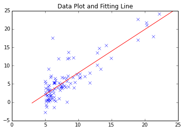
最もシンプルな勾配降下法は上記の通り.Coursera / Machine Learning 第一回の課題はこれで全く問題ない.もとめたFitting lineは,次の通りである.
但し,より大規模なデータ,複雑なデータ分析における収束性や局所最小点への対応を考えると,実績があるモジュールを使いたくなるケースも想定される.
scipy.optimize.minimize()を使ってみる
Scipyには最適化のために,実にいろいろ関数が実装されている.
http://docs.scipy.org/doc/scipy/reference/optimize.html
今回はこの中から,「パラメータを参照する関数を最小化する」機能をもつ**scipy.optimize.minimize()**を用いることにした.ドキュメントから説明を抜粋する.
scipy.optimize.minimize (fun, x0, args=(), method=None, jac=None, hess=None, hessp=None, bounds=None, constraints=(), tol=None, callback=None, options=None)
parameters
- fun : callable
Objective function. - x0 : ndarray
Initial guess. - args : tuple, optional
Extra arguments passed to the objective function and its derivatives (Jacobian, Hessian). - method : str or callable, optional
Type of solver. Should be one of
-- ‘Nelder-Mead’
-- ‘Powell’
-- ‘CG’
-- ‘BFGS’
-- ‘Newton-CG’
-- ‘L-BFGS-B’
-- ‘TNC’
-- ‘COBYLA’
-- ‘SLSQP’
-- ‘dogleg’
-- ‘trust-ncg’
-- custom - a callable object
If not given, chosen to be one of BFGS, L-BFGS-B, SLSQP - jac : bool or callable, optional
(以下,省略)
あまり目にしたことがない計算手法がリストされていて,内容をよく知らないながらも心強い.まず,簡単な数式でテストした.
import scipy.optimize as spo
def fun1(x):
	ans = (x[0] - 1.5) ** 2 + (x[1] - 2.5) ** 2

	return ans

def fun1_grad(x):
	dx = np.zeros(2)
	dx[0] = 2 * x[0] - 3
	dx[1] = 2 * x[1] - 5

	return dx

x_init = np.array([1.0, 1.0])   # initial value

res1 = spo.minimize(fun1, x_init, method='BFGS', jac=fun1_grad, \
            options={'gtol': 1e-6, 'disp': True})
これで,$f =(x_0 - 1.5) ^2 + (x_1 - 2.5) ^2$ を最小化する $x = [1.5, 2.5]$ が求まる.
Courseraの課題に対しては,以下のようにした.まず,コスト関数,導関数のwrapperを用意.
def compute_cost_sp(theta):
    global xmat, ymat
    j = compute_cost(theta, xmat, ymat)

    return j

def compute_grad_sp(theta):
    global xmat, ymat
    j_grad = compute_grad(theta, xmat, ymat)

    return j_grad
これは,引数 (xmat, ymat) を省いて探索を行うパラメータが "theta" であることを明示することを目的としている."theta"のみを引数とする関数,導関数を渡して,scipy.optimize.minimize()を呼び出す.(グローバル変数を使うことになってしまっていますが...)
    theta_ini = np.zeros(2)
    res1 = spo.minimize(compute_cost_sp, theta_ini, method='BFGS', \
         jac=compute_grad_sp, options={'gtol': 1e-6, 'disp': True})
    print ' theta.processed =', res1.x
実はwrapperを書かなくてもargs で必要なデータ(xmat, ymat)を渡すことができるのだがここは「調整パラメータ」を明確にすることを意識した.計算結果は以下の通り.
# 自前のGradient Descent (iteration = 2000回)
theta =     -3.788,      1.182
# scipy.optimize.minimize() の結果
Optimization terminated successfully.
         Current function value: 4.476971
         Iterations: 4
         Function evaluations: 6
         Gradient evaluations: 6
 theta.processed = [-3.89578088  1.19303364]
確率的(stochastic)にしてみる
ここからは,課題に含まれない(勝手に行った)応用編である.Deep Learningで多用される,確率的勾配降下法(Stochastic Gradient Descent) の「お試し」をしてみた.
def stochastic_g_d(theta, alpha, sample_ratio, num_iters):
    # calculate the number of sampling data (original size * sample_ratio)
    sample_num = int(len(ymat) * sample_ratio)

    m = len(ymat)      # number of train examples (total)
    n = np.size(xmat) / len(xmat)
    j_history = np.zeros(num_iters)

    for iter in range(num_iters):
        xs = np.zeros((sample_num, n)) ; ys = np.zeros(sample_num)

        for i in range(sample_num):
            myrnd = np.random.randint(m)
            xs[i,:] = xmat[myrnd,]
            ys[i]   = ymat[myrnd]

        delta_t = alpha * compute_grad(theta, xs, ys)
        theta = theta - delta_t
        j_history[iter] = compute_cost(theta, xmat, ymat)

    return theta, j_history
上記コードでは,Train Data のサンプリングから最小化までを自分のコードで行ったが,Train Dataをサンプリング後,scipy.optimize.minimize() で解を求めることももちろん可能.
S.G.D.(Stochastic Gradient Descent) の詳しい説明は参考文献(web記事)を参照されたい.
「肝」となるのは,コスト関数,導関数を計算するのに使うデータをサンプリングするところにある.
今回のTrain Data数は,100にも満たない小サイズなので,S.G.D.を用いる必要は全くないのだが,規模の大きいデータを扱うケースでは,計算効率が大きく向上することができるとのこと.
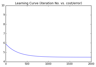
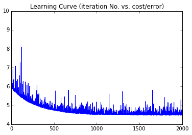
Learning Curveを作図すると以下のようになった.(横軸:ループ計算の回数,縦軸:コスト,通常の勾配降下法と確率的勾配法.)
Gradient Descent Method (reference)
Stochastic Gradient Descent (sampling/whole data= 0.3)
Couseraで課題をこなしながら,自分で範囲を広げていけるのが楽しい.今回のMachine Learningもまだ受講途中だが,Machine Learningの次に何を受講しようか?についていろいろ考え中である.最近は有料コースの"Specialization"が増えてきているが,無料コースの中にもいろいろ興味をひかれるものがある.(結構,時間が取られてしまいますが...)
参考文献
- Cousera, Machine Learning (Stanford University)
(毎週,プログラミング課題の説明書/PDFが配布されます.) - Scipy Documentation http://docs.scipy.org/doc/scipy/reference/optimize.html
- Theano, Deep Learning Tutorial http://deeplearning.net/tutorial/
- Qiita: 【更新】確率的勾配降下法とは何か、をPythonで動かして解説するhttp://qiita.com/kenmatsu4/items/d282054ddedbd68fecb0
- (連載)機械学習 はじめよう,第16回 最適化のための勾配法
http://gihyo.jp/dev/serial/01/machine-learning/0016