はじめに
こんにちは。
私は最近MITがディープラーニング(以降 DL)の授業をYouTube上で公開しているのを知り、それを使って目下勉強中です。
下記リンクには授業内で使っているスライドと各授業のYouTube動画パスがあります。
6S.191 Introduction to Deep Learning
もちろん英語ですが、読める方はぜひ挑戦してみてください。結構面白いです!
Lab1-1
ディープラーニングを実際に実装しているソースコードが公開されているので、それの解説をしていきます(要は備忘録です)
ソースコード ⇦ 今回はpart1です!
今回の内容はTensorFlowの基本的な機能の説明です
1. tesnorflowの機能の説明
2. パーセプトロンの実装
3. 勾配降下法の実装
以上のラインナップです。
ちなみにTensorFlowはなぜTensorFlowと呼ばれるかご存知でしょうか?
Tensor(N次元のベクトルや行列)のFlow(nodeや計算)をするのでTensorFlowと言う名前らしいです!明日から友達に「TesnsorFlowの名前の由来知ってる?」でマウントを取れますね!
コードの解説
TensorFlowで次元数の確認と特定の次元数を持つ変数を作成
# 0次元
sport = tf.constant('Tennis', tf.string)
number = tf.constant(1.41421356237, tf.float64)

print("`sport` is a {}-d Tensor".format(tf.rank(sport).numpy()))
print("`number` is a {}-d Tensor".format(tf.rank(number).numpy()))
`sport` is a 0-d Tensor
`number` is a 0-d Tensor
0次元のtensorを定義しました。
これはスカラーを表しています。スカラーはただの値なので次元を持っていません。
tf.rank(変数).numpy()メソッドを使うことによって、その変数の次元数を取得することができます。
numpy()で次元数のみの取得を実現しています。rank()だけだと不要な値まで返ってきます。
また、tf.constantでは公式ドキュメントより***「Creates a constant tensor from a tensor-like object」***とあるので、
tensor型の変数を作成しているというのがわかります。第二引数でどんな型のデータを持つかを決めます。
# 1次元 = ベクトル

sports = tf.constant(["Tennis", "Basketball"], tf.string)
numbers = tf.constant([3.141592, 1.414213, 2.71821], tf.float64)

print("`sports` is a {}-d Tensor with shape: {}".format(tf.rank(sports).numpy(), tf.shape(sports)))
print("`numbers` is a {}-d Tensor with shape: {}".format(tf.rank(numbers).numpy(), tf.shape(numbers)))
`sports` is a 1-d Tensor with shape: [2]
`numbers` is a 1-d Tensor with shape: [3]
1次元のtensorを定義しました。
これはベクトルの形です。ベクトルは1次元として扱われます。tf.shape(変数)で要素数を返します。
### Defining higher-order Tensors ###

'''TODO: Define a 2-d Tensor'''
matrix = tf.constant([['Baseball', 'Softball'], ['Soccer', 'Football'], ['Tennis', 'Badminton']], tf.string)

assert isinstance(matrix, tf.Tensor), "matrix must be a tf Tensor object"
assert tf.rank(matrix).numpy() == 2
# assertについて https://codezine.jp/article/detail/12179

print("`matrix` is a {}-d Tensor with shape: {}".format(tf.rank(matrix).numpy(), tf.shape(matrix)))
`matrix` is a 2-d Tensor with shape: [3 2]
rank=次元数  shape=(行数、列数)を返す。
2次元のtensorを定義しました。
2次元のデータはマトリックス(行列)になります。形としてはリストの中にリストがある形となります。
assert関数を使うことで条件を満たしていない場合AssertionErrorを表示することができ何を満たせてないかがすぐわかるようになります。
assert 条件
例として上のコードを書き換えてみます。
### Defining higher-order Tensors ###

'''TODO: Define a 2-d Tensor'''
# matrix = tf.constant([['Baseball', 'Softball'], ['Soccer', 'Football'], ['Tennis', 'Badminton']], tf.string)
matrix = tf.constant([1, 2 ,3 ], tf.int64)

assert isinstance(matrix, tf.Tensor), "matrix must be a tf Tensor object"
assert tf.rank(matrix).numpy() == 2
# assertについて https://codezine.jp/article/detail/12179

print("`matrix` is a {}-d Tensor with shape: {}".format(tf.rank(matrix).numpy(), tf.shape(matrix)))
AssertionError                            Traceback (most recent call last)
<ipython-input-42-2e33b2575781> in <module>()
      6
      7 assert isinstance(matrix, tf.Tensor), "matrix must be a tf Tensor object"
----> 8 assert tf.rank(matrix).numpy() == 2
      9 # assertについて https://codezine.jp/article/detail/12179
     10

AssertionError:
このように次元数がクリアできてない(2次元以上ではない)のでエラーが出ています。
これは自分の書いた計算式とかがあっているや欲しいoutputが手に入っているのかエラーで教えてくれるのですごく便利なものだと思います!
'''TODO: Define a 4-d Tensor.'''
# Use tf.zeros to initialize a 4-d Tensor of zeros with size 10 x 256 x 256 x 3.
#   You can think of this as 10 images where each image is RGB 256 x 256.
# (画像の数、画像のheight, 画像のwidth, 画像のチャネル数)
images = tf.constant(tf.zeros([10, 256, 256, 3]))

assert isinstance(images, tf.Tensor), "matrix must be a tf Tensor object"
assert tf.rank(images).numpy() == 4, "matrix must be of rank 4"
assert tf.shape(images).numpy().tolist() == [10, 256, 256, 3], "matrix is incorrect shape"
4次元のtensorを定義しました。
コメントアウトでも書いてますが4次元のリストは画像データを表す際に使われます。上のコードでは10枚のRGB表記の写真(256x256)となります。
実際にどのような構造になっているかみてみます。
images
<tf.Tensor: shape=(10, 256, 256, 3), dtype=float32, numpy=
array([[[[0., 0., 0.],
         [0., 0., 0.],
         [0., 0., 0.],
         ...,
         [0., 0., 0.],
         [0., 0., 0.],
         [0., 0., 0.]],...
ちゃんと4次元のリストになっていますね。3個の要素が入ったリストが並んでいると思いますが、これはRGB(Red, Green, Blue)の値になります。それが256x256あると言うことになります。
このようにtf.zeros()を使うことで4次元のtensorを簡単に実現することができます。他にもtf.ones, tf.fill, tf.eyeなども同じようなことができます。
またリストやarrayと同じようにスライスを用いることで指定の要素にアクセスできます。
# use slices to access substensors
row_vector = matrix[1]
column_vector = matrix[:,1]
scalar = matrix[0,1]

print("`row_vector`: {}".format(row_vector.numpy()))
print("`column_vector`: {}".format(column_vector.numpy()))
print("`scalar`: {}".format(scalar.numpy()))
`row_vector`: [b'Soccer' b'Football']
`column_vector`: [b'Softball' b'Football' b'Badminton']
`scalar`: b'Softball'
Tesnor型同士の計算
Tensor型同士の簡単な計算方法をみていきます。
# Create the nodes in the graph, and initialize values
a = tf.constant(15)
b = tf.constant(61)

# Add them!
c1 = tf.add(a,b)
c2 = a + b # TensorFlow overrides the "+" operation so that it is able to act on Tensors
print(c1)
print(c2)
tf.Tensor(76, shape=(), dtype=int32)
tf.Tensor(76, shape=(), dtype=int32)
### Defining Tensor computations ###

# Construct a simple computation function
def func(a,b):
  '''TODO: Define the operation for c, d, e, f (use tf.add, tf.subtract, tf.multiply, tf.divide).'''
  c = tf.add(a,b)
  d = tf.subtract(b,1)
  e = tf.multiply(c,d)
  f = tf.divide(e, a)
  return f

# Consider example values for a,b
a, b = 1.5, 2.5
# Execute the computation
f_out = func(a,b)
print(f_out)
tf.Tensor(4.0, shape=(), dtype=float32)
このようにtensorflowのメソッドを使って計算を行うこともできますし、tesnorflowは+, -, *, /の計算オペレーションもカバーしているのでこれを使っても計算できます!
パーセプトロンの実装
そして今からが面白いところですね!tensorflowライブラリを使ってディープニューラルネットワークの考えの基になっているパーセプトロンを実装してみましょう!

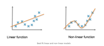
パーセプトロンはすごくシンプルなものでy=ax+bの式に非常に似ています。ベクトルxをインプットとして受け取り、各xの要素に重みw1をかけて(複数output時は行列)、全てを足してバイアスw0を足すことで結果zを出します。そして最後に非線形関数(例:sigmoid)を適用して、出力zを出します。非線形関数を使う理由としてはそのままでいくと直線の出力しか出せなくて、分類を行う時直線でしか分類が行えなくなるので使います!イメージはこんな感じですね!より細かく分類することを可能にしています!
パーセプトロンの式も書いておきます。
y=g(w_{0}+\sum_i^mx_{i}w_{i})
アウトプットが一つの単純パーセプトロンの式です。i=1からはじまります(書き方がわからなかったです)。
gは非線形関数を表しています。
今回は複数のアウトプットを求めますので下の式になります。
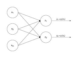
z_{i}=w_{0,i}+\sum_j^mx_{j}w_{j,i}
やることはほとんど変わりません。変わったところはoutputを複数出すために重みとバイアスが増えて行列になっているところですね。
それではpythonで実装していきましょう!
ここではクラス作成して使っています。tensorflowだけを使って実装することもできますが、クラス、関数を作ることで可読性や汎用性のあるコードにすることができますので、おすすめです!
では、コード全体をみましょう!
# Simple perceptron
### Defining a network Layer ###

# n_output_nodes: number of output nodes
# input_shape: shape of the input
# x: input to the layer

class OurDenseLayer(tf.keras.layers.Layer):
  def __init__(self, n_output_nodes):
    super(OurDenseLayer, self).__init__() # 親クラスのコンストラクタを呼び出し
    self.n_output_nodes = n_output_nodes

  def build(self, input_shape):
    d = int(input_shape[-1])
    # Define and initialize parameters: a weight matrix W and bias b
    # parameter is random at first
    self.W = self.add_weight('weight', shape=[d, self.n_output_nodes]) # note the dimensionality
    self.b = self.add_weight('bias', shape=[1, self.n_output_nodes]) # note the dimensionality

  def call(self, x):
    '''TODO: define the operation for z (hint: use tf.matmul)'''
    z = tf.matmul(x, self.W) + self.b # TODO

    '''TODO: define the operation for out (hint: use tf.sigmoid)'''
    y = tf.sigmoid(z) # TODO
    return y

# Since layer parameters are initialized randomly, we will set a random seed for reproducibility
tf.random.set_seed(1)
layer = OurDenseLayer(3) # 3 outputs
layer.build((1,2)) # 1行、2列 → inputが2つある
x_input = tf.constant([[1,2.]], shape=(1,2))
y = layer.call(x_input)

# test the output
print(y.numpy()) # should output 3 answers
mdl.lab1.test_custom_dense_layer_output(y)
[[0.2697859  0.45750412 0.66536945]]
[PASS] test_custom_dense_layer_output
True
となります。アウトプットを見てわかる通り今回は3つのアウトプットを出すようにしたので3つでてきてます。
では順番に解説していきます。クラスの解説は今回の目的とは外れるのでしません。
まずコンストラクタ__init__でアウトプットがいくつかを指定できるようにします。
build()メソッドでインプットの形を受け取ります。インプットはベクトルなので(1, n)となります。
それを使い必要な重みとバイアスを初期化しています。
最後にcall()メソッドで計算を行なっています。tf.matmulでベクトルxと重みとバイアスの行列を計算しています。
そして最後にシグモイド関数(tf.sigmoid)を適用してアウトプットyを出しています。
ちなみにcallメソッドはobj.call()かobj()で呼び出すことができます。
パーセプトロンのアルゴリズムは非常にシンプルでわかりやすかったと思います!今はインプット層とアウトプット層しかありませんでしたが、
これをもっと多層にしていけば最終的にディープニューラルネットワーク(Fully Connected Neural Network)になります!
続いてSequential modelを使っても実装してみます。
# Sequential model using Model API
### Defining a model using subclassing ###

from tensorflow.keras import Model
from tensorflow.keras.layers import Dense

class SubclassModel(tf.keras.Model):
  # Define the model's layer
  def __init__(self, n_output_nodes):
    super(SubclassModel, self).__init__()
    '''TODO: Our model consists of a single Dense layer. Define this layer.'''
    self.dense_layer = Dense(n_output_nodes, activation='sigmoid') # アウトプット層のobj作成

  # call function to define the Model's forward pass
  def call(self, inputs):
    return self.dense_layer(inputs).numpy()

n_output_nodes = 3
model = SubclassModel(n_output_nodes)

x_input = tf.constant([[1,2.]], shape=(1,2))

print(model.call(x_input))
[[0.5607363 0.6566898 0.1249697]]
Sequentialは次回以降も頻繁に使われますが、ネットワーク層を順番に定義していくことができ非常に読みやすく使いやすいです。
今回はアウトプット層のみですが、より多層にすることも可能です。
以上でパーセプトロンの実装例は終わりです!このアルゴリズムの理解は今後のニューラルネットワークの理解に非常に役に立ちますのでぜひ理解してください!
勾配降下法の実装
勾配降下法ニューラルネットワークの学習において非常に重要になってくる考えです。学習フェーズではLoss関数(例:relu)を使用して、予測されyと正解yのlossを出します。lossは小さければ誤差がない(正解に近い)のでそれを使って勾配降下法のアルゴリズムで重みを最適化していきます。要は重みに対するLossの微分をとって最適な重みを探そうと言うものです。
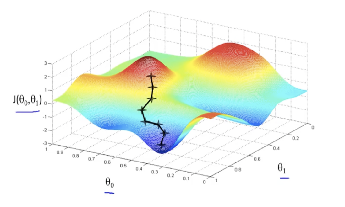
new W=W-n\frac{\partial L}{\partial W}
微分を求めることで傾きを知れるのでlossが小さくなる向きがわかります(つまりマイナス方向に移動したい)。nはlearning rateと呼ばれるもので実際にどのくらいの距離を移動するかを決定しています。そして移動した分をWから引いて新しいWを取得します。これを繰り返すことで図のようにlossが小さい方へと移動し精度の高い予測ができるようになります。簡単ですが以上が勾配降下法の説明です。これの派生で色々な手法や勾配降下方の問題点もありますので興味ある方は調べてみてください。
では、まずtensorflowを使って簡単な勾配(微分)を計算してみます。ここではわかりにくいですが***確率的勾配降下法(SGD)***が使われています。
GradientTapeを使ってしてみます。
# First, we will look at how we can compute gradients using GradientTape and access them for computation.
### Gradient computation with GradientTape ###

# y = x^2
# Example: x = 3.0
x = tf.Variable(3.0)

# Initiate the gradient tape
with tf.GradientTape() as tape:
  # Define the function
  y = x * x
# Access the gradient -- derivative of y with respect to x
dy_dx = tape.gradient(y,x)

assert dy_dx.numpy() == 6.0
print(dy_dx)
tf.Tensor(6.0, shape=(), dtype=float32)
with tf.GradientTape()の中で関数を定義します。
tape.gradient(y,x)でxに対するyの勾配を求めます。
簡単に実装することができました!これは自分でも微分できるものなので正しく計算できているか、ぜひ確認してください。
次にlossが本当に小さくなっていくのかをみていきます。ここではxをランダムに決めて正解x=4に勾配降下法を使って近づけていきます。
パーセプトロンを使っての計算などはせずに単純に定義したxが正解xに近づけるかをみていきます。
# how actually we use gradient to minimize loss
### Function minimization with automatic differentiation and SGD ###

# initialize a random value for our initial x
x = tf.Variable([tf.random.normal([1])])
print('Initializing x={}'.format(x.numpy()))

learning_rate = 1e-2 # learning rate for SGD
history = []
# Define the target value
x_f = 4

# We will run SGD for a number of iterations. At each iteration, we compute the loss,
#   compute the derivative of the loss with respect to x, and perform the SGD update.
for i in range(500):
  with tf.GradientTape() as tape:
    '''TODO: define the loss as described above'''
    # loss = tf.keras.metrics.mean_squared_error(x_f, x)
    loss = (x_f - x)**2

   # loss minimization using gradient tape
   grad = tape.gradient(loss, x) # compute the derivative of the loss with respect to x
   new_x = x - learning_rate*grad # sgd update
   x.assign(new_x) # update the  value of x
   history.append(x.numpy()[0])

  # plot the evolution of x as we optimize towards x_f
  plt.plot(history)
  plt.plot([0,500], [x_f,x_f])
  plt.legend(('Predicted', 'True'))
  plt.xlabel('Iteration')
  plt.ylabel('x value')
Initializing x=[[-1.1771784]]

実際に正解に近づいてるのがわかりますね。やっていることは先程説明した通りで、勾配降下法で最適なxを見つけて、xをアップデートしてより正解xに近づくようにしこれを500回繰り返してます。グラフで見てわかるように正解にどんどん近づいていってます。
以上で勾配降下法の説明終わりです!
まとめ
以上でtensorflowの説明を終わります。今回は学習や予測を通しての実装はしませんでしたが、今回の書いたコードをうまく組み合わせば、自分で予測を行うようプログラムできると思います。興味あればぜひやってみてください!
パーセプトロンの理解は非常に重要ですので押さえておいてください。また、勾配降下法は学習において最重要なので、理屈を知っておくことは非常に重要です。
では、次回は音楽自動生成をRNNでしていきます!
間違いや理解しにくいところがあればコメントしていただけると幸いです。