[Meep] オープンソースのFDTDシミュレータで、リング共振器のシミュレーションを試してみよう

はじめに

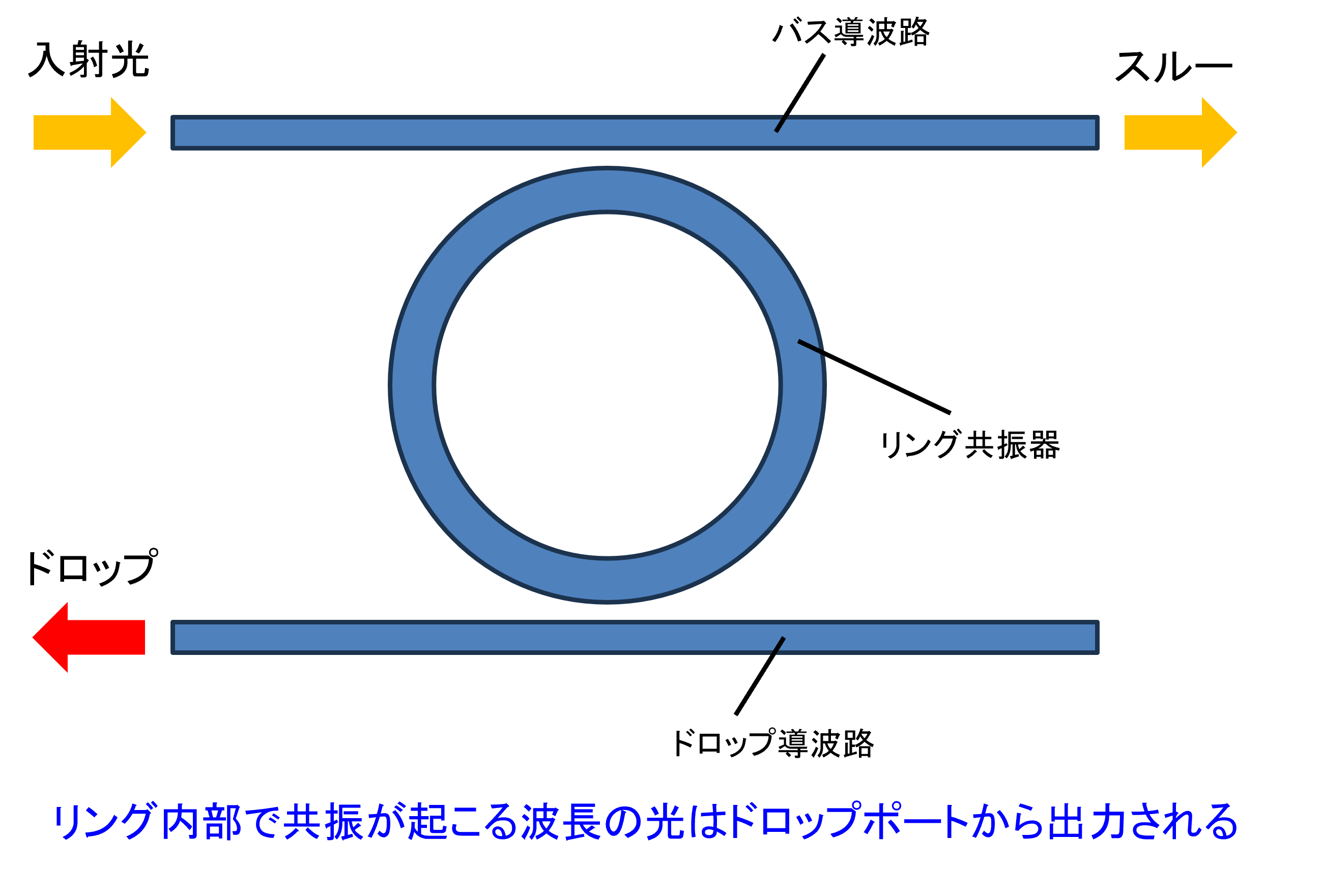
オープンソースの FDTD シミュレータである Meep を用いて、導波路付きリング共振器（バス導波路＋リング＋ドロップ導波路）の光学シミュレーションを行ってみます。
本記事では、3 次元 FDTD 計算により、リング共振器の透過スペクトル・ドロップスペクトルを計算し、さらに共振時の電場分布を可視化する一連の流れを Python スクリプトで実装します。

Meepに関してはこちらをご参照(https://meep.readthedocs.io/en/master/)

スクリプト全体

このスクリプトは、Meep を用いて導波路付きリング共振器の 3 次元 FDTD シミュレーションを行うものです。
バス導波路、リング共振器、ドロップ導波路を幾何構造として定義し、EigenModeSource により導波路の基本モードをブロードバンドで励起しています。
計算領域の端部には PML 境界条件を設定し、透過ポートおよびドロップポートにフラックスモニタを配置することで、波長依存の透過スペクトルとドロップスペクトルを取得しています。
シミュレーション実行後には、得られたフラックスデータからリング共振器のスペクトル特性を可視化しています。
さらに、計算終了時点での z=0 平面における電場 Ez の分布を取得し、リング共振器周辺の電場の様子を 2 次元プロットとして表示しています。

注)計算の設定次第では計算時間が非常にかかります。

import meep as mp
import numpy as np
import matplotlib.pyplot as plt


def main():
    # === Parameters ===
    n = 3.4
    w = 0.5
    h = 0.22
    r = 10.0
    gap = 0.05
    dpml = 2.0
    pad = 2.0
    sx = 2 * (r + w + gap + pad + dpml)
    sy = 2 * (r + w + gap + pad + dpml)
    sz = h + 2 * dpml + 1.0  # Ensure enough space in the z-direction
    cell = mp.Vector3(sx, sy, sz)

    # === Geometry setup (all z-centers are set to 0) ===
    bus_y = 0
    ring_center_y = w + gap + r
    drop_y = 2 * r + 2 * gap + 2 * w

    geometry = [
        mp.Block(
            size=mp.Vector3(mp.inf, w, h),
            center=mp.Vector3(0, bus_y, 0),
            material=mp.Medium(index=n)
        ),
        mp.Block(
            size=mp.Vector3(mp.inf, w, h),
            center=mp.Vector3(0, drop_y, 0),
            material=mp.Medium(index=n)
        ),
        mp.Cylinder(
            radius=r + w / 2, height=h,
            center=mp.Vector3(0, ring_center_y, 0),
            material=mp.Medium(index=n)
        ),
        mp.Cylinder(
            radius=r - w / 2, height=h,
            center=mp.Vector3(0, ring_center_y, 0),
            material=mp.Medium(index=1.0)
        ),
    ]

    # === Source settings ===
    fcen = 0.64
    df = 0.1
    nfreq = 50
    src = [mp.EigenModeSource(
        src=mp.GaussianSource(fcen, fwidth=df),
        center=mp.Vector3(-0.5 * sx + dpml + 1, 0, 0),
        size=mp.Vector3(0, w, h),
        direction=mp.X,
        eig_band=1,
        eig_parity=mp.ODD_Z,
    )]

    # === Monitor locations (centered at z=0) ===
    trans_pt = mp.Vector3(0.5 * sx - dpml - 1, 0, 0)
    drop_pt = mp.Vector3(0.5 * sx - dpml - 1, ring_center_y, 0)

    # === Simulation definition ===
    sim = mp.Simulation(
        cell_size=cell,
        geometry=geometry,
        sources=src,
        resolution=40,
        boundary_layers=[mp.PML(dpml)],
        dimensions=3,
    )

    # === Flux monitors ===
    trans_flux = sim.add_flux(fcen, df, nfreq,
        mp.FluxRegion(center=trans_pt, size=mp.Vector3(0, w, h)))
    drop_flux = sim.add_flux(fcen, df, nfreq,
        mp.FluxRegion(center=drop_pt, size=mp.Vector3(0, w, h)))

    # === Run simulation ===
    sim.use_output_directory()
    sim.run(
        mp.at_beginning(mp.output_epsilon),
        mp.at_every(1 / fcen / 20, mp.output_efield_z),
        until_after_sources=1000
    )

    # === Retrieve spectrum ===
    flux_freqs = mp.get_flux_freqs(trans_flux)
    trans_data = mp.get_fluxes(trans_flux)
    drop_data = mp.get_fluxes(drop_flux)
    wavelengths = [1 / f for f in flux_freqs]

    # === Plot transmission/drop spectrum ===
    plt.figure()
    plt.plot(wavelengths, trans_data, label="Transmission")
    plt.plot(wavelengths, drop_data, label="Drop")
    plt.xlabel("Wavelength (μm)")
    plt.ylabel("Flux")
    plt.title("Ring Resonator Spectrum")
    plt.grid(True)
    plt.legend()
    plt.gca().invert_xaxis()
    plt.tight_layout()
    plt.show()

    # === Ez field visualization (2D slice at z = 0) ===
    ez_center = mp.Vector3(0, ring_center_y, 0)
    ez_size = mp.Vector3(sx, sy, 0)  # 2D slice (thickness 0 in z)
    ez_data = sim.get_array(center=ez_center, size=ez_size, component=mp.Ez)

    extent = [-0.5 * sx, 0.5 * sx,
              ring_center_y - 0.5 * sy, ring_center_y + 0.5 * sy]

    plt.figure()
    plt.imshow(np.rot90(ez_data), interpolation='spline36', cmap='RdBu',
               extent=extent)
    plt.colorbar(label="Ez")
    plt.title("Ez Field Distribution (z = 0 plane)")
    plt.xlabel("x (μm)")
    plt.ylabel("y (μm)")
    plt.tight_layout()
    plt.show()


if __name__ == "__main__":
    main()

参考リンク

※本記事は筆者個人の見解であり、所属組織の公式見解を示すものではありません。

問い合わせ

光学シミュレーションソフトの導入や技術相談、
設計解析委託をお考えの方はサイバネットシステムにお問合せください。

光学ソリューションサイトについては以下の公式サイトを参照：
👉 光学ソリューションサイト(サイバネット)

光学分野のエンジニアリングサービスについては以下の公式サイトを参照：
👉 光学エンジニアリングサービス(サイバネット)