問い合わせフォームのご連絡
この記事の内容についてのご質問や、
Ansys(Lumerical / HFSS など)の使い方相談はもちろん、
フリーソフト・OSSを使ったシミュレーションや解析の技術的なご相談も受け付けています。
「この設定で合ってる?」「この解析、どう進めるのがよい?」
「商用ソフトとフリーソフト、どう使い分けるべき?」
といったレベル感でも問題ありません。
気軽にこちらの問い合わせフォームからご連絡ください👇
はじめに
前回の記事
ではTorchOpticsの紹介をしました。
今回は試用してみたので、ご紹介します。
【TorchOptics】DOE / SLM を用いたフーリエ面強度最適化
― Phase-only 最適化(①)と Amplitude+Phase 最適化(②)の比較 ―
今回の計算では、TorchOptics + PyTorch を用いた
フーリエ面強度分布の逆設計ーInverse Designーの2つの計算事例を紹介します。
今回の設定ではレンズと入射光を同じ位置において、レンズの焦点距離fだけ離れた位置での像分布を計算してみます。

事例①:四角形像の分布を得るための入射光の位相分布最適化
今回のターゲット像

事例①ではターゲット像の対称性が良いので入射光の位相のみを変えて最適化を目指してみます。
事例②:にこちゃんマーク像の分布を得るための入射光の振幅と位相分布最適化
今回のターゲット像

事例②では非対称性が大きいので入射光の位相だけではなく、振幅も変えないとターゲット像を作るのは無理でしょう。
実際のスクリプト
事例①
import math
import torch
import torchoptics
from torchoptics import Field, System
from torchoptics.elements import Lens, PhaseModulator

import numpy as np
import matplotlib.pyplot as plt

shape = 512
spacing = 10e-6
wavelength = 700e-9
f = 200e-3

# ★重要:DOE(PhaseModulator)とレンズを同一面(z=0)に置く
z_lens = 0.0
# ★フーリエ面=レンズ焦点面(レンズから距離 f)
z_fourier = f

iters = 800
lr = 0.05

device = "cuda" if torch.cuda.is_available() else "cpu"

torchoptics.set_default_spacing(spacing)
torchoptics.set_default_wavelength(wavelength)

# target (square in Fourier plane)
fill_ratio = 0.25
side = int(fill_ratio * shape)
I_tgt = torch.zeros((shape, shape), device=device)
c = shape // 2
h = side // 2
I_tgt[c-h:c+h, c-h:c+h] = 1.0
I_tgt = I_tgt / (I_tgt.mean() + 1e-12)

# learnable phase parameter
phi_raw = torch.nn.Parameter(torch.zeros((shape, shape), device=device))

def wrapped_phase(p):
    return 2 * math.pi * torch.sigmoid(p)

lens = Lens(shape, f, z=z_lens).to(device)

# input plane wave at the DOE/lens plane
input_field = Field(torch.ones((shape, shape), device=device)).to(device)
opt = torch.optim.Adam([phi_raw], lr=lr)

def intensity(field):
    if hasattr(field, "intensity"):
        return field.intensity()
    return field.abs() ** 2

def corr_loss(I, T):
    I0 = I - I.mean()
    T0 = T - T.mean()
    corr = (I0*T0).mean() / (I0.std()+1e-12) / (T0.std()+1e-12)
    return 1 - corr

def plot_intensity_with_linecuts(I_torch, title="", log10=True, eps=1e-6,
                                 clip_percentiles=(1, 99.5), normalize="max"):
    I = I_torch.detach().float().cpu().numpy()

    if normalize == "max":
        I = I / (I.max() + 1e-12)
    elif normalize == "mean":
        I = I / (I.mean() + 1e-12)

    H, W = I.shape
    cy, cx = H // 2, W // 2

    if log10:
        I_show = np.log10(I + eps)
        vmin, vmax = None, None
        cbar_label = "log10(I + eps)"
    else:
        vmin, vmax = np.percentile(I, clip_percentiles)
        I_show = I
        cbar_label = "I (clipped)"

    cut_x = I[cy, :]
    cut_y = I[:, cx]

    fig = plt.figure(figsize=(12, 4))

    ax0 = fig.add_subplot(1, 3, 1)
    im = ax0.imshow(I_show, origin="lower", vmin=vmin, vmax=vmax)
    ax0.set_title(title if title else "Intensity")
    ax0.set_xlabel("x (pixel)")
    ax0.set_ylabel("y (pixel)")
    cb = plt.colorbar(im, ax=ax0, fraction=0.046, pad=0.04)
    cb.set_label(cbar_label)

    ax1 = fig.add_subplot(1, 3, 2)
    ax1.plot(cut_x)
    ax1.set_title("Center line cut (y=center)")
    ax1.set_xlabel("x (pixel)")
    ax1.set_ylabel("I")
    ax1.grid(True, alpha=0.3)
    ax1.set_yscale("log")
    ax1.set_ylim(1e-6, 1.0)

    ax2 = fig.add_subplot(1, 3, 3)
    ax2.plot(cut_y)
    ax2.set_title("Center line cut (x=center)")
    ax2.set_xlabel("y (pixel)")
    ax2.set_ylabel("I")
    ax2.grid(True, alpha=0.3)
    ax2.set_yscale("log")
    ax2.set_ylim(1e-6, 1.0)

    plt.tight_layout()
    plt.show()

for it in range(1, iters + 1):
    phi = wrapped_phase(phi_raw)

    phase_mod = PhaseModulator(phi).to(device)
    system = System(phase_mod, lens).to(device)

    # ★フーリエ面は z=f
    out_field = system.measure_at_z(input_field, z=z_fourier)

    I = intensity(out_field)
    I = I / (I.mean() + 1e-12)

    loss = torch.mean((I - I_tgt) ** 2) + 0.5 * corr_loss(I, I_tgt)

    opt.zero_grad(set_to_none=True)
    loss.backward()
    opt.step()

    if it % 50 == 0 or it == 1:
        print(f"iter {it:4d} | loss {loss.item():.6e}")

with torch.no_grad():
    phi = wrapped_phase(phi_raw)
    phase_mod = PhaseModulator(phi).to(device)
    system = System(phase_mod, lens).to(device)

    out_field = system.measure_at_z(input_field, z=z_fourier)
    out_field.visualize(title="Achieved intensity @ Fourier plane (z=f)", vmax=1)

    plt.figure()
    plt.imshow(phi.detach().cpu().numpy(), origin="lower")
    plt.title("Optimized phase [rad] (0..2π)")
    plt.colorbar()
    plt.tight_layout()
    plt.show()

    I = intensity(out_field)
    plot_intensity_with_linecuts(
        I, title="Fourier plane intensity (z=f)",
        log10=True, eps=1e-6, normalize="max"
    )
事例②
import math
import torch
import torchoptics
from torchoptics import Field, System
from torchoptics.elements import Lens, PhaseModulator

import numpy as np
import matplotlib.pyplot as plt

# ----------------------------
# 0) parameters
# ----------------------------
shape = 512
spacing = 10e-6
wavelength = 700e-9
f = 200e-3

# ★重要:レンズを z=0、フーリエ面を z=f にする
z_lens = 0.0
z_fourier = f

iters = 2000
lr = 0.03

device = "cuda" if torch.cuda.is_available() else "cpu"
print("device:", device)

torchoptics.set_default_spacing(spacing)
torchoptics.set_default_wavelength(wavelength)

# ----------------------------
# 1) target (smiley intensity in Fourier plane) 反転なし
# ----------------------------
def make_smiley_target(shape, device="cpu",
                       face_radius_ratio=0.40,
                       eye_offset_ratio=(0.16, 0.14),   # dyを上げると目が上へ
                       eye_radius_ratio=0.035,
                       mouth_radius_ratio=0.23,
                       mouth_thickness_ratio=0.020,
                       mouth_y_offset_ratio=-0.06,      # 負で下
                       mouth_angle_deg=(210, 330),
                       blur_sigma_px=2.0):

    H = W = shape
    yy, xx = torch.meshgrid(
        torch.arange(H, device=device),
        torch.arange(W, device=device),
        indexing="ij"
    )
    cy = (H - 1) / 2.0
    cx = (W - 1) / 2.0

    x = (xx - cx)
    y = (yy - cy)  # ★反転しない

    r = torch.sqrt(x**2 + y**2)

    face_R = face_radius_ratio * shape
    face = (r <= face_R).float()

    eye_R = eye_radius_ratio * shape
    dx = eye_offset_ratio[0] * shape
    dy = eye_offset_ratio[1] * shape

    # ★dy>0で「上」に移動(origin="lower" 表示と整合)
    eye1 = (torch.sqrt((x - dx)**2 + (y - dy)**2) <= eye_R).float()
    eye2 = (torch.sqrt((x + dx)**2 + (y - dy)**2) <= eye_R).float()

    my = mouth_y_offset_ratio * shape
    mouth_R = mouth_radius_ratio * shape
    mouth_t = mouth_thickness_ratio * shape

    rr = torch.sqrt(x**2 + (y - my)**2)
    ring = ((rr >= (mouth_R - mouth_t/2)) & (rr <= (mouth_R + mouth_t/2))).float()

    ang = torch.atan2((y - my), x)
    ang_deg = (ang * 180.0 / math.pi) % 360.0

    a0, a1 = mouth_angle_deg
    if a0 <= a1:
        arc = ((ang_deg >= a0) & (ang_deg <= a1)).float()
    else:
        arc = ((ang_deg >= a0) | (ang_deg <= a1)).float()

    mouth = ring * arc

    I = 0.25 * face + 1.0 * (eye1 + eye2) + 0.9 * mouth

    # blur(これが無いと難易度が跳ねる)
    if blur_sigma_px and blur_sigma_px > 0:
        sigma = float(blur_sigma_px)
        k = int(6*sigma + 1) | 1
        ax = torch.arange(k, device=device) - k//2
        g = torch.exp(-(ax**2) / (2*sigma**2))
        g = g / g.sum()

        I_ = I[None, None, :, :]
        g1 = g[None, None, :, None]
        g2 = g[None, None, None, :]
        I_ = torch.nn.functional.conv2d(I_, g2, padding=(0, k//2))
        I_ = torch.nn.functional.conv2d(I_, g1, padding=(k//2, 0))
        I = I_[0, 0]

    I = I / (I.mean() + 1e-12)
    return I

I_tgt = make_smiley_target(shape, device=device)

plt.figure(figsize=(4,4))
plt.imshow(I_tgt.detach().cpu().numpy(), origin="lower")
plt.title("Target intensity: Smiley")
plt.colorbar()
plt.tight_layout()
plt.show()

# ----------------------------
# 2) learnable amplitude + phase (SLM at z=0 = lens plane)
# ----------------------------
amp_raw = torch.nn.Parameter(torch.zeros((shape, shape), device=device))
phi_raw = torch.nn.Parameter(torch.zeros((shape, shape), device=device))

def wrapped_phase(p):
    return 2 * math.pi * torch.sigmoid(p)

def bounded_amp(a):
    # 0..1
    return torch.sigmoid(a)

# optics (lens at z=0)
lens = Lens(shape, f, z=z_lens).to(device)

opt = torch.optim.Adam([amp_raw, phi_raw], lr=lr)

# ----------------------------
# 3) helpers
# ----------------------------
def intensity(field):
    if hasattr(field, "intensity"):
        return field.intensity()
    return field.abs() ** 2

def corr_loss(I, T):
    I0 = I - I.mean()
    T0 = T - T.mean()
    corr = (I0 * T0).mean() / (I0.std() + 1e-12) / (T0.std() + 1e-12)
    return 1 - corr

def tv_loss(x):
    dx = x[:, 1:] - x[:, :-1]
    dy = x[1:, :] - x[:-1, :]
    return (dx.abs().mean() + dy.abs().mean())

# 強度そのものより sqrt(I) の方が見た目に効きやすいことが多い
def mse_on_sqrtI(I, T, eps=1e-8):
    return torch.mean((torch.sqrt(I + eps) - torch.sqrt(T + eps))**2)

# regularization weights
w_corr = 0.2
w_tv   = 3e-2
w_l2a  = 1e-3

# ----------------------------
# 4) optimization loop
# ----------------------------
for it in range(1, iters + 1):
    amp = bounded_amp(amp_raw)
    phi = wrapped_phase(phi_raw)

    # 入力は平面波 * 振幅
    input_field = Field(torch.ones((shape, shape), device=device)).to(device)

    # SLM:位相はPhaseModulator、振幅はFieldに掛ける
    # (Fieldの data に掛ける)
    input_field = Field(amp * input_field.data).to(device)

    phase_mod = PhaseModulator(phi).to(device)
    system = System(phase_mod, lens).to(device)

    out_field = system.measure_at_z(input_field, z=z_fourier)
    I = intensity(out_field)
    I = I / (I.mean() + 1e-12)

    # loss(sqrt強度MSE + corr + 正則化)
    l_mse  = mse_on_sqrtI(I, I_tgt)
    l_corr = corr_loss(I, I_tgt)
    l_tv   = tv_loss(amp)
    l_l2a  = ((amp - 0.5)**2).mean()

    loss = l_mse + w_corr * l_corr + w_tv * l_tv + w_l2a * l_l2a

    opt.zero_grad(set_to_none=True)
    loss.backward()
    opt.step()

    if it % 100 == 0 or it == 1:
        print(f"iter {it:4d} | loss {loss.item():.3e} | mse {l_mse.item():.3e} | corr {l_corr.item():.3e} | tv {l_tv.item():.3e}")

# ----------------------------
# 5) visualize
# ----------------------------
with torch.no_grad():
    amp = bounded_amp(amp_raw)
    phi = wrapped_phase(phi_raw)

    input_field = Field(torch.ones((shape, shape), device=device)).to(device)
    input_field = Field(amp * input_field.data).to(device)

    phase_mod = PhaseModulator(phi).to(device)
    system = System(phase_mod, lens).to(device)

    out_field = system.measure_at_z(input_field, z=z_fourier)
    out_field.visualize(title="Achieved intensity @ Fourier plane (z=f)", vmax=1)

    I = intensity(out_field)
    I = I / (I.mean() + 1e-12)

    plt.figure(figsize=(12,4))
    plt.subplot(1,3,1)
    plt.imshow(amp.detach().cpu().numpy(), origin="lower")
    plt.title("Optimized amplitude (0..1)")
    plt.colorbar()

    plt.subplot(1,3,2)
    plt.imshow(phi.detach().cpu().numpy(), origin="lower")
    plt.title("Optimized phase [rad] (0..2π)")
    plt.colorbar()

    plt.subplot(1,3,3)
    plt.imshow(I_tgt.detach().cpu().numpy(), origin="lower")
    plt.title("Target (Smiley)")
    plt.colorbar()

    plt.tight_layout()
    plt.show()

    # 見た目比較用(sqrt強度)
    plt.figure(figsize=(10,4))
    plt.subplot(1,2,1)
    plt.imshow(torch.sqrt(I + 1e-8).detach().cpu().numpy(), origin="lower")
    plt.title("sqrt(Achieved I)")
    plt.colorbar()
    plt.subplot(1,2,2)
    plt.imshow(torch.sqrt(I_tgt + 1e-8).detach().cpu().numpy(), origin="lower")
    plt.title("sqrt(Target I)")
    plt.colorbar()
    plt.tight_layout()
    plt.show()
シミュレーション結果
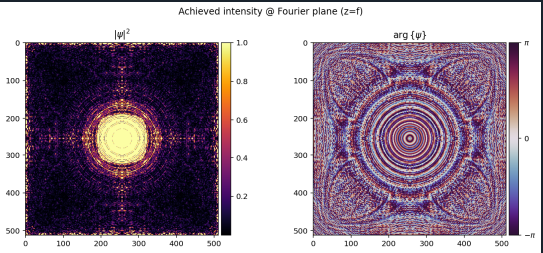
事例①
こちらが得られた像の強度分布です。強度が特に強い部分だけに着目すれば、四角っぽい形状ができています。
それでこちらが入射光の位相分布です。

事例②
こちらが得られた強度分布です。

局所的に分布が強いポイントが出ており、全体的に真っ暗になってます。
ダイナミックレンジが大きいので、得られた強度分布のルートをとってみましょう

にこちゃんマークが出てきました。
こちらが入射光の振幅分布と位相分布です。

入射面のサイズはどう決まっているか?
コード中では次のように設定しています:
shape   = 512
spacing = 10e-6  # 10 µm
これは、
- ピクセル数:512 × 512
- ピクセルピッチ:10 µm
を意味します。
したがって、入射面の物理サイズは:
Lin=N⋅Δx=512×10μm=5.12mm
つまり、DOE / SLM の有効開口は約 5 mm × 5 mm です。
フーリエ面のピクセルサイズ
離散フーリエ変換の関係から、
フーリエ面のピクセルサイズは次式で与えられます:
- 入射面サイズ:約 5 mm
- フーリエ面サイズ:約 14 mm
同じ 512×512 の配列でも、
入射面とフーリエ面では物理サイズが全く異なります。
まとめ
今回はTorchOpticsを用いて、ターゲット像を設定し、入射光の①位相分布を変える逆設計と②入射光の振幅と位相を変える逆設計を試してみました。
paraxial近似前提なので、高NAには適用できませんが、回折光学素子の逆設計問題を解くうえで非常に有用そうです。
※本記事は筆者個人の見解であり、所属組織の公式見解を示すものではありません。
問い合わせ
光学シミュレーションソフトの導入や技術相談、
設計解析委託をお考えの方はサイバネットシステムにお問合せください。
光学ソリューションサイトについては以下の公式サイトを参照:
👉 [光学ソリューションサイト(サイバネット)]
https://www.cybernet.co.jp/optical/
光学分野のエンジニアリングサービスについては以下の公式サイトを参照:
👉 [光学エンジニアリングサービス(サイバネット)]