この記事は,Pythonそのものの使い方かDeepLearningの仕組みまで,1から細かく学習した際のメモ書きとスライドのまとめです.
単純パーセプトロン(AND真偽値表の学習)
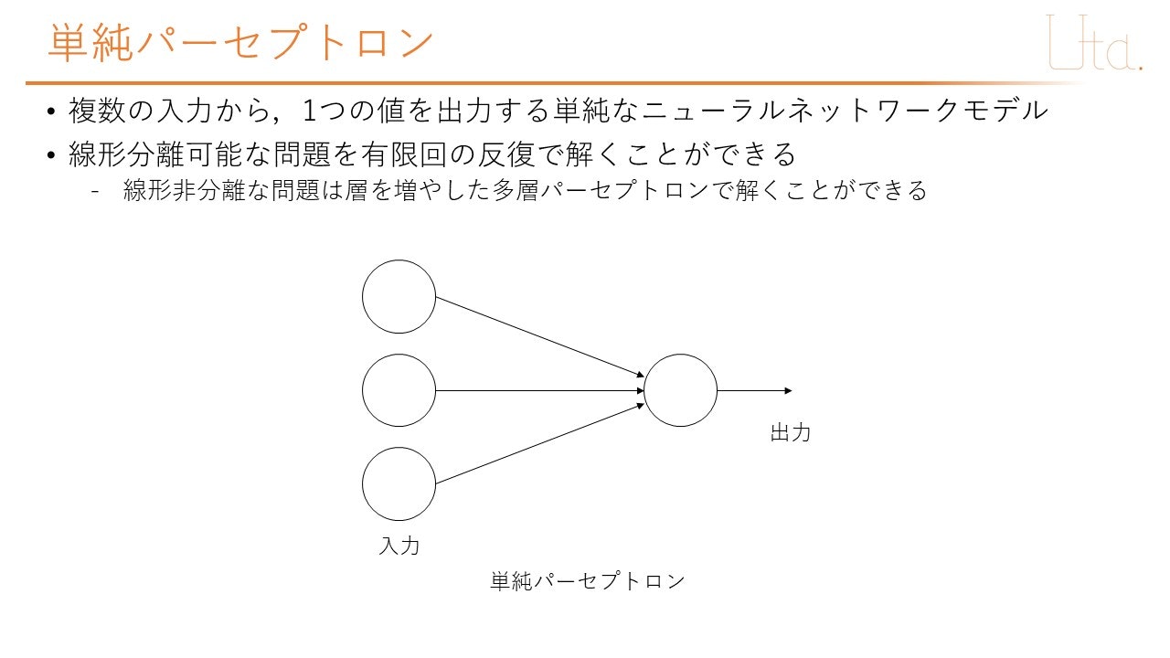
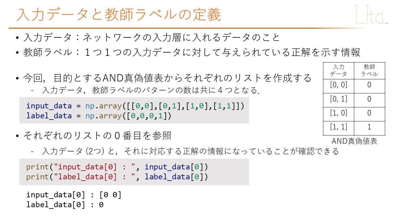
今回は,単純パーセプトロン(Perceptron)を用いて,AND真偽値表の出力を学習させることを目指す.AND真理値表とは,入力の2つが共に1である時のみ1を出力するものである.
| x1 | x2 | y |
|---|---|---|
| 0 | 0 | 0 |
| 0 | 1 | 0 |
| 1 | 0 | 0 |
| 1 | 1 | 1 |
はじめに
前提として,Pythonの基本的な使い方(クラスを扱える程度)を理解していることとして話を進める.
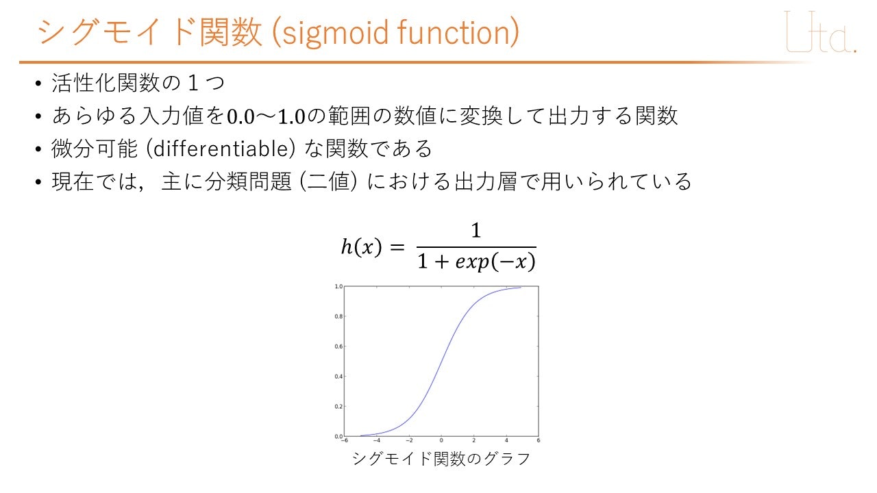
ライブラリであるNumpyを扱うが,この分野でよく使い,複雑な挙動をするnumpy.dot()と,ニューラルネットワークで一般的に使用されるシグモイド関数については,以下に解説する.
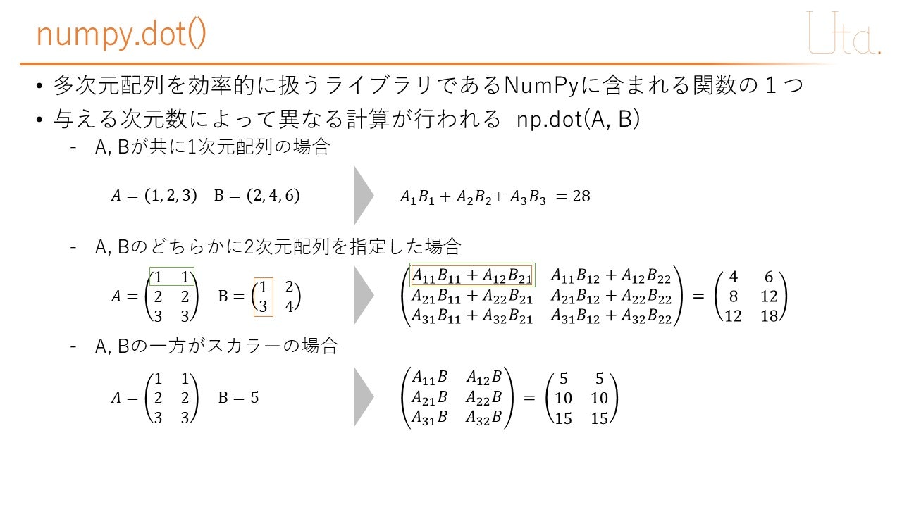
上記のnumpy.dot()の挙動については,以下のコードを用いて確認ができる.
import numpy as np
# A,Bが共に1次元配列の場合
A = np.array([1,2,3])
B = np.array([2,4,6])
ans1 = np.dot(A,B)
print("ans1 = ", ans1)

# A,Bのどちらかに2次元配列を指定した場合
A = np.array([[1,1],[2,2],[3,3]])
B = np.array([[1,2],[3,4]])
ans2 = np.dot(A,B)
print("ans2 = \n", ans2)

# A,Bの一方がスカラーの場合
A = np.array([[1,1],[2,2],[3,3]])
B = 5 #スカラー
ans3 = np.dot(A,B)
print("ans3 = \n", ans3)
実行結果
ans1 =  28
ans2 =
 [[ 4  6]
 [ 8 12]
 [12 18]]
ans3 =
 [[ 5  5]
 [10 10]
 [15 15]]
モデルの作成
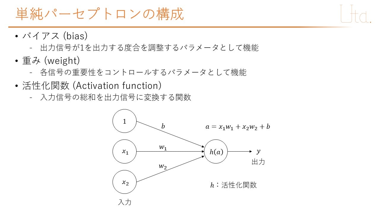
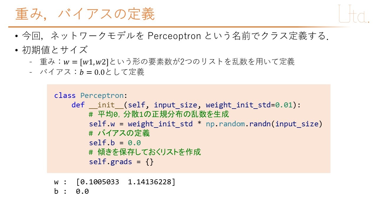
重み (weight)
今回は,入力層から出力層へ向かう重みをリストwで定義した.入力層から出力層へ向かう重みはx1→a,x2→aへ向かう2つである.したがって,w1=w[0],w2=w[1]で定義した.
バイアス (bias)
今回は,バイアスが1つなので,そのまま変数でbを定義した.
プログラム
import numpy as np
import matplotlib.pyplot as plt
%matplotlib inline
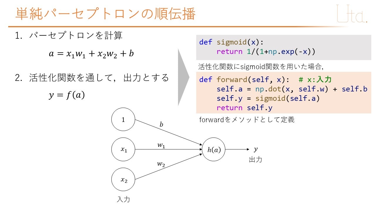
# ネットワークモデルに必要な活性化関数の定義(sigmoid関数)
def sigmoid(x):
return 1/(1+np.exp(-x))
def sigmoid_grad(x):
return (1.0 - sigmoid(x))*sigmoid(x)
# ネットワークモデルの定義(単純パーセプトロン)
class Perceptron:
def __init__(self, input_size, weight_init_std=0.01):
# 平均0,分散1の正規分布の乱数を生成
self.w = weight_init_std * np.random.randn(input_size)
# バイアスの定義
self.b = 0.0
# 傾きを保存しておくリストを作成
self.grads = {}
def forward(self, x): # x:入力
self.a = np.dot(x, self.w) + self.b
self.y = sigmoid(self.a)
return self.y
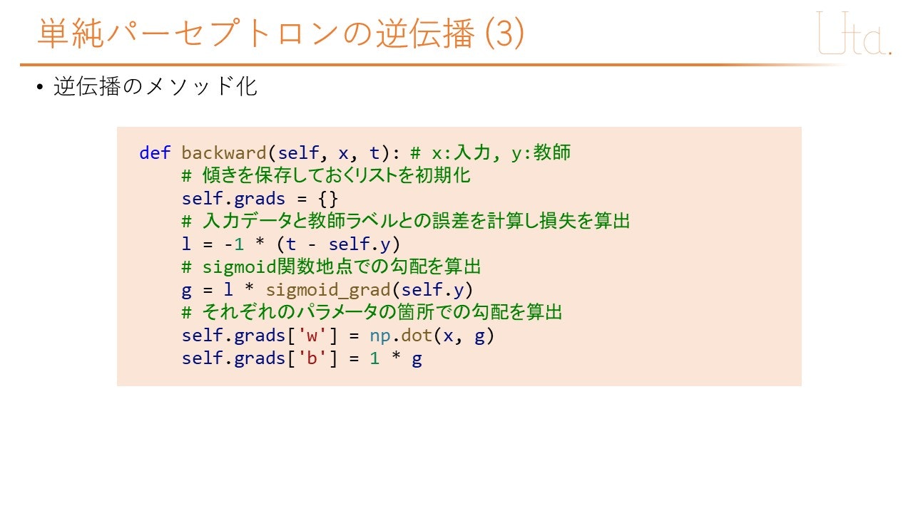
def backward(self, x, t): # x:入力, y:教師
# 傾きを保存しておくリストを初期化
self.grads = {}
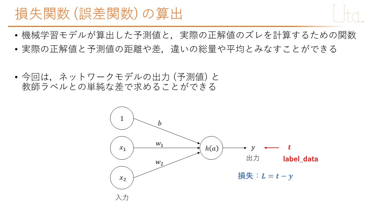
# 入力データと教師ラベルとの誤差を計算し損失を算出
l = -1 * (t - self.y)
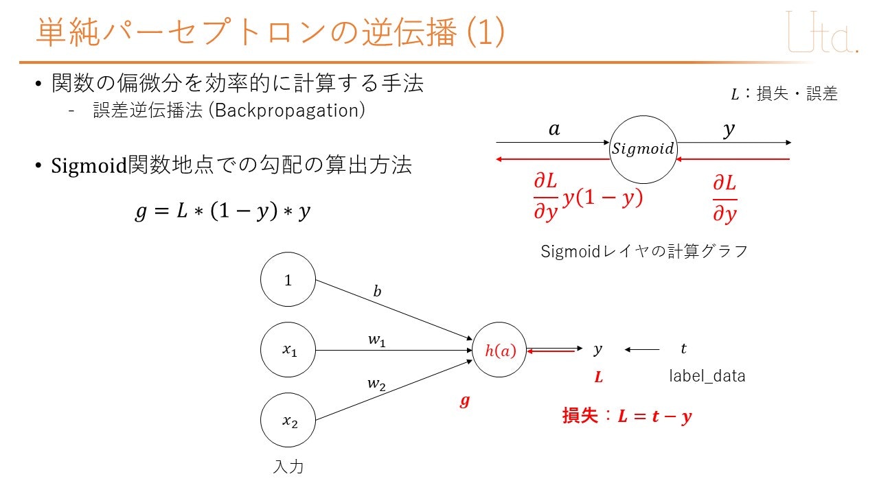
# sigmoid関数地点での勾配を算出
g = l * sigmoid_grad(self.y)
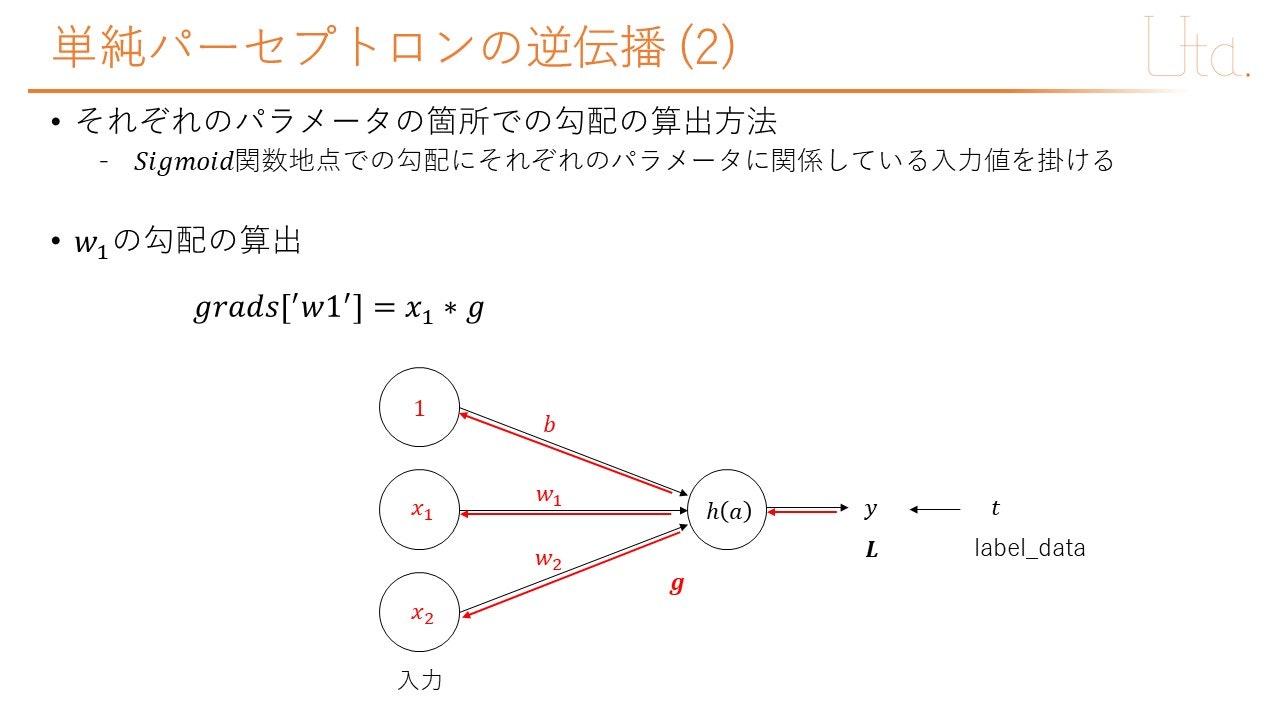
# それぞれのパラメータの箇所での勾配を算出
self.grads['w'] = np.dot(x, g)
self.grads['b'] = 1 * g
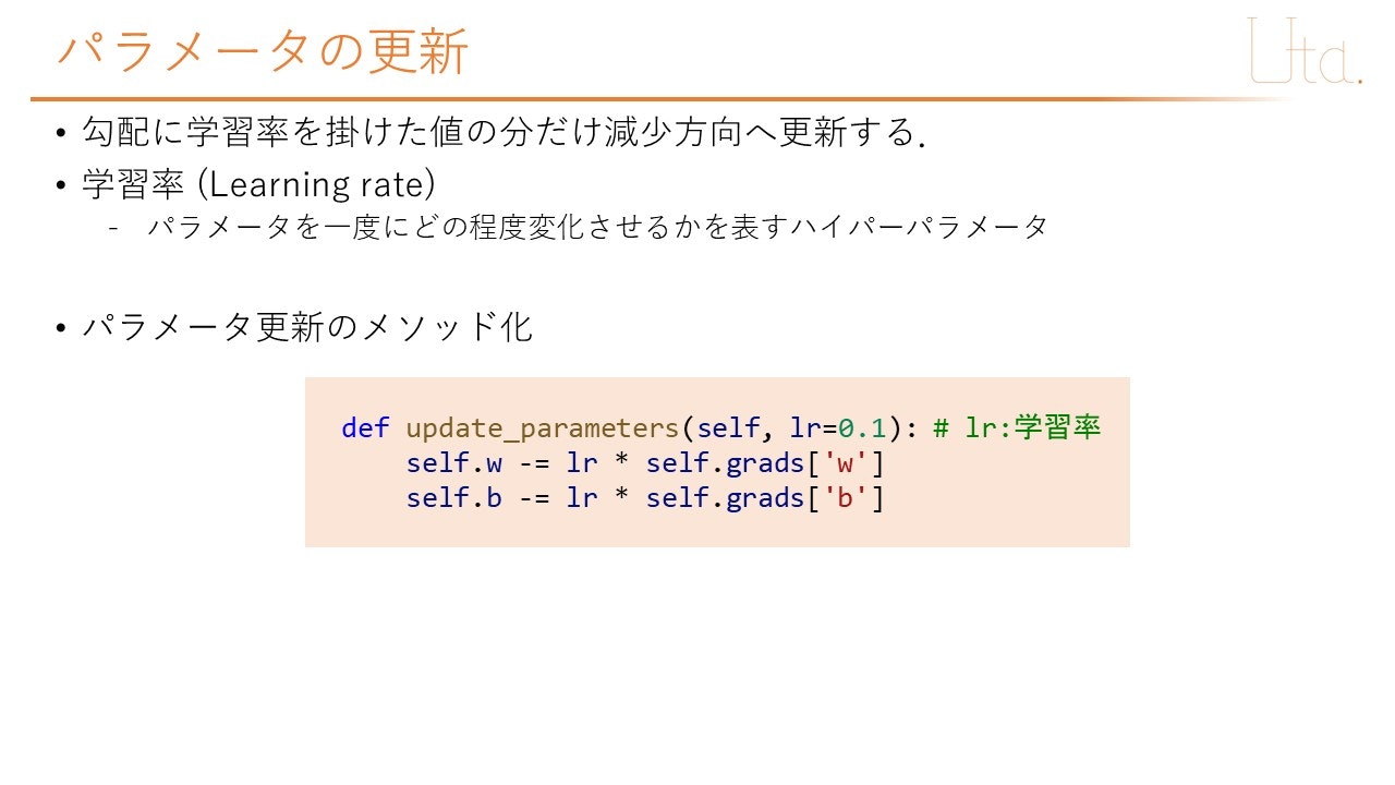
def update_parameters(self, lr=0.1): # lr:学習率
self.w -= lr * self.grads['w']
self.b -= lr * self.grads['b']
# モデルパラメータを表示させる関数
def display_model_parameters(model):
print("w : ", model.w, "b : ", model.b)
if __name__=="__main__":
# AND回路の学習を行うための入力データと教師ラベルの定義
input_data = np.array([[0,0],[0,1],[1,0],[1,1]])
label_data = np.array([0,0,0,1])
# モデルの作成
input_size = 2
model = Perceptron(input_size=input_size, weight_init_std=1)
display_model_parameters(model)
# 学習パラメータの指定
num_train_data = 4
epoch_num = 5000
learning_rate = 0.1
train_loss_list = []
# 学習回数分繰り返す
for epoch in range(1, epoch_num+1, 1):
sum_loss = 0.0
for i in range(0, num_train_data, 1):
# 学習1回に用いるinputデータとlabelを抽出
input = input_data[i]
label = label_data[i]
y_pred = model.forward(input)
model.backward(input, label)
model.update_parameters(lr=learning_rate)
sum_loss += np.power(y_pred - label ,2)
train_loss_list.append(sum_loss/4)
print("epoch : {}, loss : {}" .format(epoch, sum_loss/4))
display_model_parameters(model)
#正解率の算出
print("=============検証==============")
cnt_correct = 0
cnt_all = 0
tolerance = 0.1 #許容範囲の設定
for i in range(0,len(input_data)):
y = model.forward(input_data[i])
print("input_data : {}, y : {}".format(input_data[i], y))
label = label_data[i]
if label-tolerance < y and y < label+tolerance:
cnt_correct += 1
cnt_all += 1
accuracy = cnt_correct/cnt_all
print("accuracy : ", accuracy)
#学習推移グラフの描画
plt.plot(range(len(train_loss_list)), train_loss_list)
plt.xlabel('epoch')
plt.ylabel('train_loss')
plt.show()
実行結果
w :  [ 0.04044971 -0.44445208] b :  0.0
epoch : 1, loss : 0.2755540842082671
epoch : 2, loss : 0.25938457825839456
epoch : 3, loss : 0.24498575229365263
epoch : 4, loss : 0.23200674181546946
            <中略>
epoch : 4997, loss : 2.064664218037121e-05
epoch : 4998, loss : 2.0638412153166655e-05
epoch : 4999, loss : 2.063018704184902e-05
epoch : 5000, loss : 2.0621966842505977e-05
w :  [10.46145475 10.46020368] b :  -15.977199379164789
=============検証==============
input_data : [0 0], y : 1.1513050864149548e-07
input_data : [0 1], y : 0.004001821880506588
input_data : [1 0], y : 0.004006811506167369
input_data : [1 1], y : 0.992927608306417
accuracy :  1.0
