本記事では、速度チャンネルマップ (velocity channel map) を作ります。
今回も例によって国立天文台の FUGIN プロジェクトで得られた野辺山45m電波望遠鏡の CO 輝線のアーカイブデータを使用します。データは
http://jvo.nao.ac.jp/portal/nobeyama/
から
FGN_03100+0000_2x2_12CO_v1.00_cube.fits
をダウンロードします (重いです)。
また、 Spitzer の 8.0 µm データを使用します。
https://irsa.ipac.caltech.edu/data/SPITZER/GLIMPSE/images/I/1.2_mosaics_v3.5/GLON_30-53/
から GLM_03000+0000_mosaic_I4.fits をダウンロードしました。
速度チャンネルマップは、aplpy.FITSFigure の subplot を指定すれば比較的簡単に作れます (綺麗にするのは少し難しいです)。
まず必要なものを import します。
from astropy.io import fits
import numpy as np
import matplotlib.pyplot as plt
import aplpy
from matplotlib import cm
そして、積分強度を作る & fits を切り取って軽くするために、前回の記事 などで紹介した関数を定義します。
def xyv2ch(x, y, v, w):#km/s
    x_ch, y_ch, v_ch   = w.wcs_world2pix(x, y, v*1000.0, 0)
    x_ch = int(round(float(x_ch), 0))
    y_ch = int(round(float(y_ch), 0))
    v_ch = int(round(float(v_ch), 0))
    return x_ch, y_ch, v_ch

def xy2ch(x, y, w):
    x_ch, y_ch   = w.wcs_world2pix(x, y, 0)
    x_ch = int(round(float(x_ch), 0))
    y_ch = int(round(float(y_ch), 0))
    return x_ch, y_ch

def v2ch(v, w):#km/s
    x_tempo, y_tempo, v_tempo   = w.wcs_world2pix(0, 0, 0, 0)
    x_ch, y_ch, v_ch   = w.wcs_world2pix(x_tempo, y_tempo, v*1000.0, 0)
    v_ch = int(round(float(v_ch), 0))
    return v_ch

def ch2v(ch, w):#km/s
    x, y, v   = w.wcs_pix2world(0, 0, ch, 0)
    return v/1000.0

def del_header_key(header, keys): # headerのkeyを消す
    import copy
    h = copy.deepcopy(header)
    for k in keys:
        try:
            del h[k]
        except:
            pass
    return h

def make_new_hdu_integ_ch(hdu, v_start_ch, v_end_ch, w): # 積分強度のhduを作る
    data = hdu.data
    header = hdu.header
    new_data = np.nansum(data[v_start_ch:v_end_ch], axis=0)*header["CDELT3"]/1000.0
    header = del_header_key(header, ["CRVAL3", "CRPIX3", "CRVAL3", "CDELT3", "CUNIT3", "CTYPE3", "CROTA3", "NAXIS3"])
    header["NAXIS"] = 2
    new_hdu = fits.PrimaryHDU(new_data, header)
    return new_hdu

def xy_cut(fits_name, x_start, x_end, y_start, y_end):
    from astropy.io import fits
    from astropy.wcs import WCS

    save_name = fits_name[:-5]+".xy_cut.fits"
    hdu = fits.open(fits_name)
    h = hdu[0].header
    d = hdu[0].data
    w = WCS(h)
    if d.ndim==3:
        x_start_ch, y_start_ch, v_tempo = xyv2ch(x_start, y_start, 0.0, w)
        x_end_ch, y_end_ch, v_tempo = xyv2ch(x_end, y_end, 0.0, w)
        if x_start_ch<0 or y_start_ch<0 or x_end_ch>h["NAXIS1"]-2 or y_end_ch>h["NAXIS2"]-2:
            print("x_start_ch, x_end_ch = ", x_start_ch, x_end_ch)
            print("y_start_ch, y_end_ch = ", y_start_ch, y_end_ch)
            print("out of fits.")
            return
        d = d[:, y_start_ch:y_end_ch+1, x_start_ch:x_end_ch+1] # +1 してます
    elif d.ndim==2:
        x_start_ch, y_start_ch = xy2ch(x_start, y_start, w)
        x_end_ch, y_end_ch = xy2ch(x_end, y_end, w)
        if x_start_ch<0 or y_start_ch<0 or x_end_ch>h["NAXIS1"]-2 or y_end_ch>h["NAXIS2"]-2:
            print("x_start_ch, x_end_ch = ", x_start_ch, x_end_ch)
            print("y_start_ch, y_end_ch = ", y_start_ch, y_end_ch)
            print("out of fits.")
            return
        d = d[y_start_ch:y_end_ch+1, x_start_ch:x_end_ch+1] # +1 してます
    else:
        print("data.ndim must be 2 or 3. ")
        return

    h['CRPIX1'] = h['CRPIX1'] - x_start_ch
    h['CRPIX2'] = h['CRPIX2'] - y_start_ch

    new_fits = fits.PrimaryHDU(d, h)
    new_fits.writeto(save_name, overwrite=True)
    return
xy_cut を使用します。fits がそもそも重くない方はスキップしても大丈夫です。
fits_name = "FGN_03100+0000_2x2_12CO_v1.00_cube.fits"
mapcenter_x, mapcenter_y, mapsize_x, mapsize_y = 30.75, 0.0, 0.5, 0.5 # degree で、map の中心と幅, 高さ
x_start, x_end = mapcenter_x + mapsize_x/2.0, mapcenter_x - mapsize_x/2.0 # degree で、左-右の順で入れる
y_start, y_end =  mapcenter_y - mapsize_y/2.0, mapcenter_y + mapsize_y/2.0 # degree で、下-上の順で入れる
xy_cut(fits_name, x_start, x_end, y_start, y_end)
# FGN_03100+0000_2x2_12CO_v1.00_cube.xy_cut.fits ができる

fits_name = "GLM_03000+0000_mosaic_I4.fits"
mapcenter_x, mapcenter_y, mapsize_x, mapsize_y = 30.75, 0.0, 0.5, 0.5 # degree で、map の中心と幅, 高さ
x_start, x_end = mapcenter_x + mapsize_x/2.0, mapcenter_x - mapsize_x/2.0 # degree で、左-右の順で入れる
y_start, y_end =  mapcenter_y - mapsize_y/2.0, mapcenter_y + mapsize_y/2.0 # degree で、下-上の順で入れる
xy_cut(fits_name, x_start, x_end, y_start, y_end)
# GLM_03000+0000_mosaic_I4.xy_cut.fits ができる
ここから本題です。
パネル数やスタートする速度などを与えるとマップが出力される関数です。適当に書いた関数なので、引数が多くて使いづらいかもしれません。
def func_chmap_integ_nxm(fits_name, v_start, ch_range, color_min, color_max, mapcenter_x, mapcenter_y, mapsize_x, mapsize_y, figsize, n, m, cmap, stretch, cb_label):
    from astropy.io import fits
    from astropy.wcs import WCS
    import numpy as np
    import matplotlib
    import matplotlib.pyplot as plt
    import aplpy
    from matplotlib.colorbar import ColorbarBase
    #from mpl_toolkits.axes_grid1 import make_axes_locatable
    from matplotlib.colors import LogNorm
    import math
    plt.rcParams['xtick.direction'] = 'in'
    plt.rcParams['ytick.direction'] = 'in'

    save_name = "chmap_%.1f_kms_%ich_%ix%i"%(v_start, ch_range, n, m)
    hdu = fits.open(fits_name)[0]
    h = hdu.header
    d = hdu.data
    w = WCS(h)
    ch_start = v2ch(v_start, w)
    position_addedlabel_x, position_addedlabel_y = mapcenter_x + mapsize_x*0.1, mapcenter_y + mapsize_y*0.43 # label の位置です。調整してください。

    fig = plt.figure(figsize=figsize)

    for i in range(n*m):
        ch_start_i, ch_end_i = int(ch_start+i*ch_range), int(ch_start+(i+1)*ch_range)
        v_start, v_end = ch2v(ch_start_i, w), ch2v(ch_end_i-1, w)
        hdu_color = make_new_hdu_integ_ch(hdu, ch_start_i, ch_end_i , w)

        f = aplpy.FITSFigure(hdu_color, slices=[0], figure=fig, subplot=[0.1+(0.8/float(n)*math.floor(i%n)),0.9-(0.8/float(m)*math.floor(i/n+1)), 0.8/float(n), 0.8/float(m)], convention='wells')
        f.recenter(mapcenter_x, mapcenter_y, width=mapsize_x, height=mapsize_y)
        f.show_colorscale(vmin=color_min, vmax=color_max, cmap=cmap, stretch=stretch)
        f.ticks.set_color("k")
        v_start_label, v_end_label = ch2v(ch_start_i, w)-h["CDELT3"]/1000.0/2.0, ch2v(ch_end_i-1, w)+h["CDELT3"]/1000.0/2.0
        f.add_label(position_addedlabel_x, position_addedlabel_y, "%.1f - %.1f km s$^{-1}$"%(v_start_label, v_end_label), color="k", size=14, family='serif', weight='bold') # 速度ラベル
        if int(i/n) != (m-1):
            f.tick_labels.hide_x()
            f.axis_labels.hide_x()
        if int(i%n) != 0:
            f.tick_labels.hide_y()
            f.axis_labels.hide_y()
        print(i+1, "/", n*m)
    #fig.canvas.draw()
    ax = fig.add_subplot(1, 1, 1)
    if stretch=="log":
        cb = ColorbarBase(ax=ax, cmap=cmap, norm=LogNorm(vmin=color_min, vmax=color_max), orientation="vertical")
    else:
        cb = ColorbarBase(ax=ax, cmap=cmap, norm=matplotlib.colors.Normalize(vmin=color_min, vmax=color_max), orientation="vertical")
    cb.ax.set_position([0.92, 0.1, 0.05, 0.8])
    cb.set_label(cb_label, size=20, family="serif")
    f.save(save_name+'.png', dpi=150)
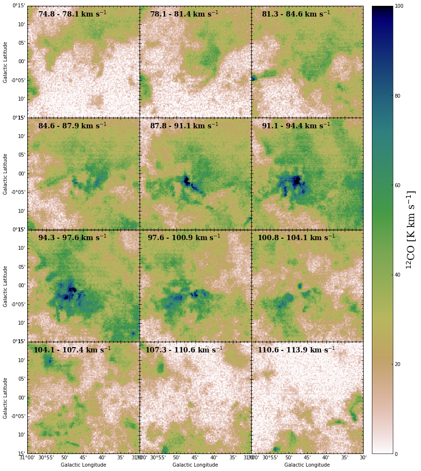
以下のように使います。
fits_name = "~/your/fits/dir/FGN_03100+0000_2x2_12CO_v1.00_cube.xy_cut.fits"
mapcenter_x, mapcenter_y, mapsize_x, mapsize_y = 30.75, 0.0, 0.5, 0.5 # degree で、map の中心と幅, 高さ
v_start = 75.0 # km/s
ch_range = 5 # 1パネルに使うチャンネル数
color_min, color_max = 0.0, 100
n, m = 3, 4 # 列数, 行数
figsize = (n*4, m*4) # figure のサイズ
cmap = cm.gist_earth_r # colormap
stretch = "linear" # linear or log
cb_label = "$^{12}$CO [K km s$^{-1}$]"
func_chmap_integ_nxm(fits_name, v_start, ch_range, color_min, color_max, mapcenter_x, mapcenter_y, mapsize_x, mapsize_y, figsize, n, m, cmap, stretch, cb_label)
カラーバーの太さや文字の大きさやその他諸々は適宜変更してください。保存形式も、 eps や pdf に変更できます。
(※ Jupyter では plot にすごい時間がかかる場合があります。どうしても遅くて我慢できない時は script にして (テキストファイルにして) ターミナルから実行してください。少し速くなります。)
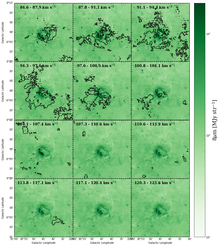
例えば、赤外線の上に CO のコントアを乗せたい場合は以下のように関数を変更します。
(速度範囲やコントアレベルは今てきとうにやっています。)
def func_chmap_integ_nxm_2(fits_name_contour, fits_name_color, v_start, ch_range, color_min,
                           color_max, mapcenter_x, mapcenter_y, mapsize_x, mapsize_y, figsize, n, m, cmap, stretch, cb_labe, levels):
    from astropy.io import fits
    from astropy.wcs import WCS
    import numpy as np
    import matplotlib
    import matplotlib.pyplot as plt
    import aplpy
    from matplotlib.colorbar import ColorbarBase
    #from mpl_toolkits.axes_grid1 import make_axes_locatable
    from matplotlib.colors import LogNorm
    import math
    plt.rcParams['xtick.direction'] = 'in'
    plt.rcParams['ytick.direction'] = 'in'

    save_name = "chmap_2_%.1f_kms_%ich_%ix%i"%(v_start, ch_range, n, m)
    hdu = fits.open(fits_name_contour)[0]
    h = hdu.header
    d = hdu.data
    w = WCS(h)
    ch_start = v2ch(v_start, w)
    position_addedlabel_x, position_addedlabel_y = mapcenter_x + mapsize_x*0.1, mapcenter_y + mapsize_y*0.43 # label の位置です。調整してください。

    fig = plt.figure(figsize=fig_size)

    for i in range(n*m):
        ch_start_i, ch_end_i = int(ch_start+i*ch_range), int(ch_start+(i+1)*ch_range)
        v_start, v_end = ch2v(ch_start_i, w), ch2v(ch_end_i-1, w)
        hdu_contour = make_new_hdu_integ_ch(hdu, ch_start_i, ch_end_i , w)

        f = aplpy.FITSFigure(fits_name_color, slices=[0], figure=fig, subplot=[0.1+(0.8/float(n)*math.floor(i%n)),0.9-(0.8/float(m)*math.floor(i/n+1)), 0.8/float(n), 0.8/float(m)], convention='wells')
        f.recenter(mapcenter_x, mapcenter_y, width=mapsize_x, height=mapsize_y)
        f.show_colorscale(vmin=color_min, vmax=color_max, cmap=cmap, stretch=stretch)
        f.ticks.set_color("k")
        v_start_label, v_end_label = ch2v(ch_start_i, w)-h["CDELT3"]/1000.0/2.0, ch2v(ch_end_i-1, w)+h["CDELT3"]/1000.0/2.0
        f.add_label(position_addedlabel_x, position_addedlabel_y, "%.1f - %.1f km s$^{-1}$"%(v_start_label, v_end_label), color="k", size=14, family='serif', weight='bold') # 速度ラベル
        f.show_contour(hdu_contour, levels=levels, colors="k")
        if int(i/n) != (m-1):
            f.tick_labels.hide_x()
            f.axis_labels.hide_x()
        if int(i%n) != 0:
            f.tick_labels.hide_y()
            f.axis_labels.hide_y()
        print(i+1, "/", n*m)
    #fig.canvas.draw()
    ax = fig.add_subplot(1, 1, 1)
    if stretch=="log":
        cb = ColorbarBase(ax=ax, cmap=cmap, norm=LogNorm(vmin=color_min, vmax=color_max), orientation="vertical")
    else:
        cb = ColorbarBase(ax=ax, cmap=cmap, norm=matplotlib.colors.Normalize(vmin=color_min, vmax=color_max), orientation="vertical")
    cb.ax.set_position([0.92, 0.1, 0.05, 0.8])
    cb.set_label(cb_label, size=20, family="serif")
    f.save(save_name+'.png', dpi=150)
fits_name_contour = "FGN_03100+0000_2x2_12CO_v1.00_cube.xy_cut.fits"
fits_name_color = "GLM_03000+0000_mosaic_I4.xy_cut.fits"
mapcenter_x, mapcenter_y, mapsize_x, mapsize_y = 30.75, 0.0, 0.5, 0.5 # degree で、map の中心と幅, 高さ
v_start = 85.0
ch_range = 5 # 1パネルに使うチャンネル数
color_min, color_max = 10.0, 2000
n, m = 3, 4 # 列数, 行数
fig_size = (n*4, m*4) # figure のサイズ
cmap = cm.Greens # colormap
stretch = "log" # linear or log
cb_label = "8$\mu$m [MJy str$^{-1}$]"
levels = np.array([1,2,3,4,5,6,7,8])*50
func_chmap_integ_nxm_2(fits_name_contour, fits_name_color, v_start, ch_range, color_min, color_max, mapcenter_x, mapcenter_y, mapsize_x, mapsize_y, figsize, n, m, cmap, stretch, cb_label, levels)
以上です。
リンク
目次