想定読者:
- 「学習域外(外挿 / OOD)」が怖いのでアラートを出したい
- kNN距離など距離ベース検知を試したが、スケールや高次元で不安がある
-
IsolationForestを聞いたことはあるが、何が嬉しいかよく分からない
この記事のゴール:
- 用語から丁寧に:学習域外(OOD) と IsolationForest の意味を理解する
- ダミーデータで:IsolationForestが距離に頼らず「学習域外っぽい入力」を検知できることを体験する
- そして:しきい値(threshold)設計の基本(q=0.99はいつ危ない?)まで持ち帰る
TL;DR(結論)
- IsolationForest は「距離」を直接使わず、**ランダムな分割で“早く孤立する点ほど異常”**とみなす異常検知手法です。
- 予測モデルとは別に「入力監視(OOD検知)」として置くと、外挿で静かに壊れるのを止めやすくなります。
- ただし
q=0.99(学習データ上位1%をアラート)は便利な初期値でも、見逃しが増えることがあります。- この記事の最小実験(seed固定)では、
-
q=0.99:FPR≈0.9% / “難しいOOD”のTPR≈0.42 -
q=0.95:FPR≈4.4% / “難しいOOD”のTPR≈0.98
となり、誤警報と見逃しのトレードオフがはっきり見えます。
-
- この記事の最小実験(seed固定)では、
1. 用語(初心者向け)
学習域外(OOD / Out-of-Distribution)
モデルが学習した入力分布(学習域)から外れた入力が来ること。
- 学習データでは見ていないユーザー層
- センサーの更新、施設差、環境変化
- データ前処理の変更 など
多くのモデルは 学習域外でも平気で予測値を出すため、「静かに壊れる」ことがよくあります。
異常検知(Anomaly Detection)
「ふだんと違う」を見つけるタスク。
OOD検知は、入力の観点では「学習データから見て“異常”」を見つけるのと近いです。
IsolationForest(ざっくり)
- ランダムに特徴量を選び、ランダムに閾値で分割する「木」をたくさん作る
- 早く孤立(isolate)する点ほど異常とみなす
- たくさんの木で平均してスコア化する
直感:
「異常は周りに仲間が少ないので、適当な切り分けでもすぐ1人にできる」
2. 距離を捨てたい理由(なぜIsolationForest?)
距離ベース(kNN距離など)は分かりやすい一方で、
- 特徴量スケールに敏感(標準化が必須になりがち)
- 高次元で距離が効きにくい(距離集中)
- “min-maxの箱”が学習域を表さない(多次元で破綻)
などの落とし穴があります。
IsolationForestは「距離」そのものを使わず、分割で孤立しやすいかという別の観点でスコアを作るため、距離が不安な場面の選択肢になります。
※注意:IsolationForestも万能ではありません(後述)。
ただ「距離以外の見方」を持てるのが価値です。
3. 最小実験:2つの“ふつう”の塊と、間に現れる“学習域外”
実験の設計(わざと分かりやすく)
- 学習データ(In):2つのガウス分布の塊(2クラスタ)
- OOD(easy):遠くに出現(見つけやすい)
- OOD(hard):2クラスタの“間”に出現(min-max範囲内にいるのに学習データが薄い)
この “hard OOD” が現場で厄介なやつです:
- 値だけ見ると「範囲内」
- でも「学習データがほぼない場所」
4. Google Colab 実行コード(上からコピペでOK)
4.1 import
import numpy as np
import pandas as pd
import matplotlib.pyplot as plt

from sklearn.ensemble import IsolationForest
from sklearn.preprocessing import StandardScaler
from sklearn.metrics import roc_auc_score
4.2 ダミーデータ生成(In / OOD easy / OOD hard)
# 再現性
rng = np.random.default_rng(0)

def make_blobs(n, centers, sigma=0.6, seed=0):
    rng = np.random.default_rng(seed)
    k = len(centers)
    idx = rng.integers(0, k, size=n)
    X = np.zeros((n, 2))
    for i, c in enumerate(centers):
        mask = (idx == i)
        X[mask] = rng.normal(loc=c, scale=sigma, size=(mask.sum(), 2))
    return X

centers = [(-2, -2), (2, 2)]

# trainは「正常(In)のみ」を仮定(novelty detectionの想定)
X_train = make_blobs(2000, centers, sigma=0.6, seed=1)

# 検証用In(同じ分布)
X_in = make_blobs(3000, centers, sigma=0.6, seed=2)

# OOD hard:2クラスタの間(min-max内だが学習データが薄い)
X_ood_center = rng.normal(loc=(0, 0), scale=0.5, size=(1500, 2))

# OOD easy:遠い場所
X_ood_far = rng.normal(loc=(5, -5), scale=0.8, size=(1500, 2))

print("train:", X_train.shape, "in:", X_in.shape, "ood_center:", X_ood_center.shape, "ood_far:", X_ood_far.shape)
4.3 前処理(標準化)+ IsolationForest 学習
IsolationForestは距離ベースではありませんが、
特徴量のスケールが大きく違うと分割が偏るので、標準化しておくのが無難です(特に多次元)。
scaler = StandardScaler().fit(X_train)

Xtr = scaler.transform(X_train)
Xin = scaler.transform(X_in)
Xc  = scaler.transform(X_ood_center)
Xf  = scaler.transform(X_ood_far)

iso = IsolationForest(
    n_estimators=400,
    contamination="auto",  # しきい値は後で自分で決めるのでautoでOK
    random_state=0
)
iso.fit(Xtr)

# scikit-learnのscore_samplesは「高いほど正常(inlier)」のスコア
# ここでは分かりやすく「大きいほど異常」にしたいので符号を反転して anomaly_score にする
anom_train = -iso.score_samples(Xtr)
anom_in    = -iso.score_samples(Xin)
anom_center= -iso.score_samples(Xc)
anom_far   = -iso.score_samples(Xf)

# 参考:分離性能(しきい値を決める前のランキング性能)
y = np.r_[np.zeros(len(anom_in)), np.ones(len(anom_center) + len(anom_far))]
score_all = np.r_[anom_in, anom_center, anom_far]
auc = roc_auc_score(y, score_all)
print("AUROC (In vs OOD) =", auc)
5. しきい値(threshold)をどう決める?:q=0.99はいつ危ない?
5.1 「q分位点」でしきい値を決める(最小構成)
まずは最小構成として、
threshold = quantile(anom_train, q)-
anom_score > thresholdならアラート
とします。
q=0.99 は「学習データの上位1%くらいをアラート」にする設計。
誤警報は少ないが、微妙なOODを見逃すことがあります。
def summarize(q):
    thr = np.quantile(anom_train, q)
    return {
        "q (train quantile)": q,
        "threshold": thr,
        "FPR on In": (anom_in > thr).mean(),
        "TPR on OOD(center=hard)": (anom_center > thr).mean(),
        "TPR on OOD(far=easy)": (anom_far > thr).mean(),
    }

summary = pd.DataFrame([summarize(0.99), summarize(0.97), summarize(0.95), summarize(0.90)])
display(summary.style.format({
    "threshold": "{:.3f}",
    "FPR on In": "{:.3f}",
    "TPR on OOD(center=hard)": "{:.3f}",
    "TPR on OOD(far=easy)": "{:.3f}",
}))
6. 図を作る(3枚)
図1:2Dで見る「異常スコア地図」+ しきい値境界(q=0.99 / q=0.95)
thr99 = np.quantile(anom_train, 0.99)
thr95 = np.quantile(anom_train, 0.95)

# グリッド(可視化用)
xlim = (-6, 6)
ylim = (-6, 6)
grid_lin = np.linspace(xlim[0], xlim[1], 240)
xx, yy = np.meshgrid(grid_lin, grid_lin)
grid = np.c_[xx.ravel(), yy.ravel()]
grid_s = scaler.transform(grid)
anom_grid = -iso.score_samples(grid_s).reshape(xx.shape)

# 表示が重いので点はサンプル
rng_plot = np.random.default_rng(1)
idx_tr = rng_plot.choice(len(X_train), size=600, replace=False)
idx_c  = rng_plot.choice(len(X_ood_center), size=400, replace=False)
idx_f  = rng_plot.choice(len(X_ood_far), size=400, replace=False)

plt.figure(figsize=(6.2, 6.2))
plt.contourf(xx, yy, anom_grid, levels=35, alpha=0.85)
cbar = plt.colorbar()
cbar.set_label("Anomaly score (-score_samples)")

# しきい値の等高線(同じスコアになる境界)
plt.contour(xx, yy, anom_grid, levels=[thr99], colors="white", linewidths=2)
plt.contour(xx, yy, anom_grid, levels=[thr95], colors="yellow", linewidths=2)

plt.scatter(X_train[idx_tr, 0], X_train[idx_tr, 1], s=8, c="black", alpha=0.6, label="train (In)")
plt.scatter(X_ood_center[idx_c, 0], X_ood_center[idx_c, 1], s=10, alpha=0.6, label="OOD center (hard)")
plt.scatter(X_ood_far[idx_f, 0], X_ood_far[idx_f, 1], s=10, alpha=0.6, label="OOD far (easy)")

plt.xlim(xlim); plt.ylim(ylim)
plt.gca().set_aspect("equal", "box")
plt.xlabel("x1"); plt.ylabel("x2")
plt.title("IsolationForest anomaly score map\nwhite=thr(q99), yellow=thr(q95)")
plt.legend(loc="upper right", fontsize=8)
plt.tight_layout()
plt.savefig("fig1_iforest_boundary.png", dpi=200)
plt.show()

print("saved: fig1_iforest_boundary.png")
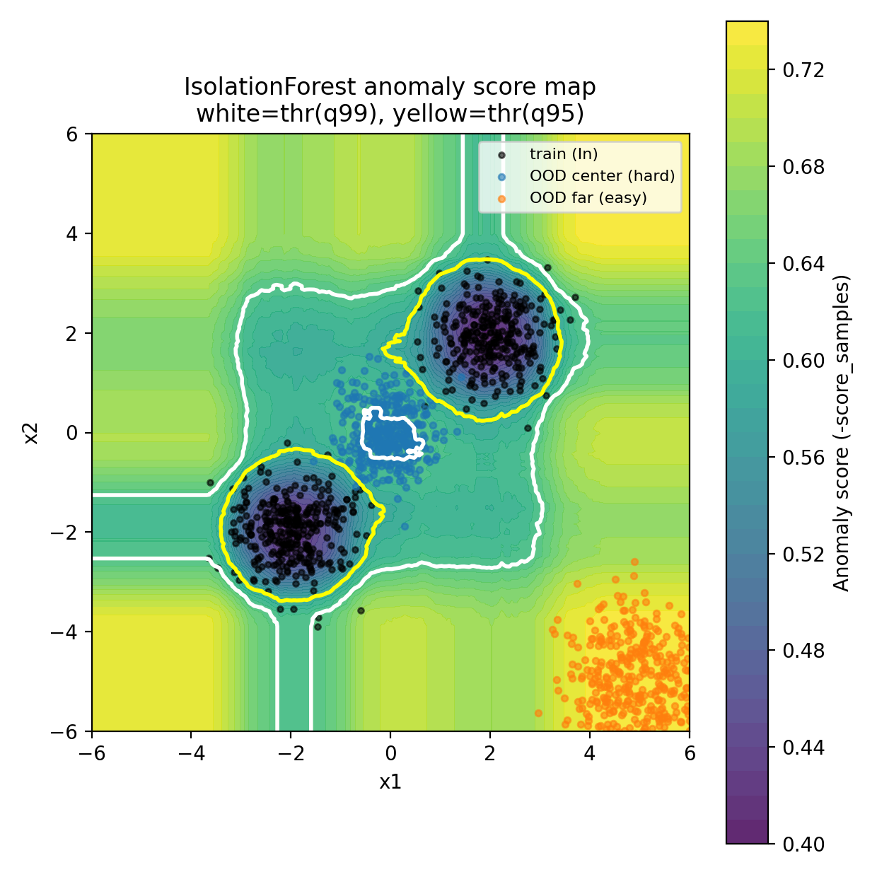
図2:誤警報(FPR)と見逃し(TPR)のトレードオフ曲線
qs = np.linspace(0.80, 0.999, 220)
fprs, tpr_center, tpr_far = [], [], []

for q in qs:
    thr = np.quantile(anom_train, q)
    fprs.append((anom_in > thr).mean())
    tpr_center.append((anom_center > thr).mean())
    tpr_far.append((anom_far > thr).mean())

fpr99 = (anom_in > thr99).mean()
tpc99 = (anom_center > thr99).mean()
tpf99 = (anom_far > thr99).mean()

fpr95 = (anom_in > thr95).mean()
tpc95 = (anom_center > thr95).mean()
tpf95 = (anom_far > thr95).mean()

plt.figure(figsize=(6.6, 4.6))
plt.plot(fprs, tpr_center, label="OOD center (hard)")
plt.plot(fprs, tpr_far, label="OOD far (easy)")

plt.scatter([fpr99], [tpc99], marker="o")
plt.scatter([fpr99], [tpf99], marker="x")
plt.text(fpr99 + 0.01, tpc99, "q=0.99", fontsize=9)

plt.scatter([fpr95], [tpc95], marker="o")
plt.scatter([fpr95], [tpf95], marker="x")
plt.text(fpr95 + 0.01, tpc95, "q=0.95", fontsize=9)

plt.xlim(0, max(fprs) * 1.05)
plt.ylim(0, 1.02)
plt.xlabel("False Positive Rate on In (FPR)")
plt.ylabel("True Positive Rate on OOD (TPR)")
plt.title("Threshold trade-off: lower threshold catches hard OOD\nbut increases false alarms")
plt.legend()
plt.tight_layout()
plt.savefig("fig2_tradeoff_curve.png", dpi=200)
plt.show()

print("saved: fig2_tradeoff_curve.png")
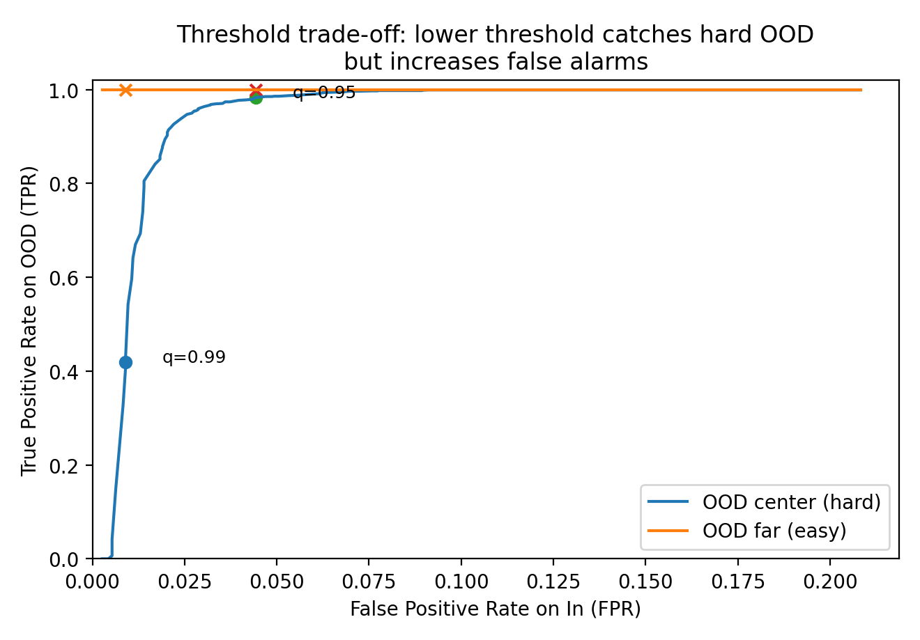
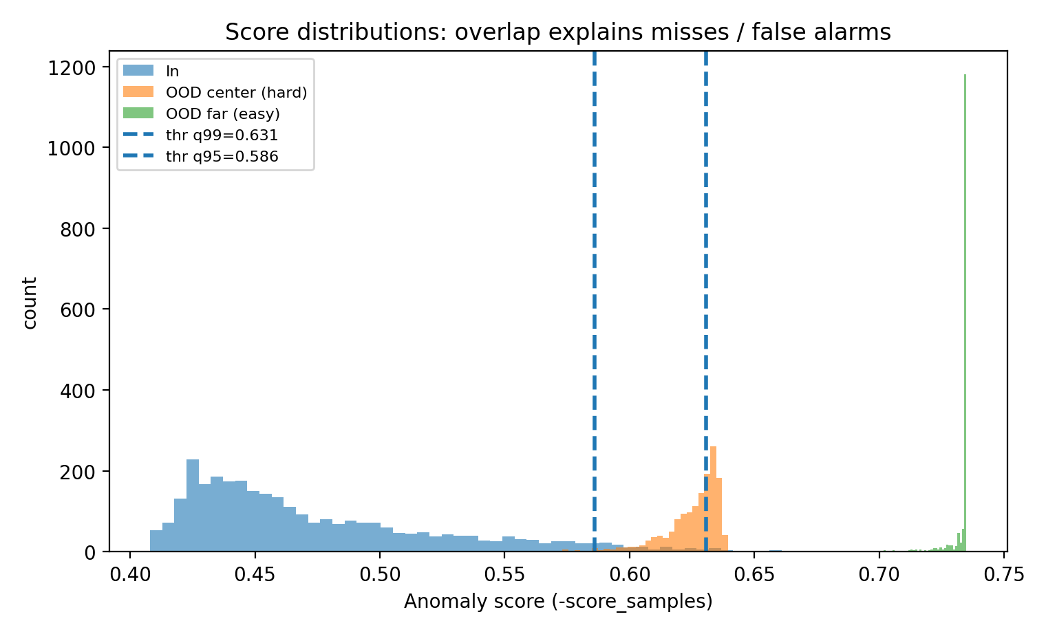
図3:スコア分布(重なりが“見逃し”を生む)
plt.figure(figsize=(7.6, 4.6))
plt.hist(anom_in, bins=60, alpha=0.6, label="In")
plt.hist(anom_center, bins=60, alpha=0.6, label="OOD center (hard)")
plt.hist(anom_far, bins=60, alpha=0.6, label="OOD far (easy)")
plt.axvline(thr99, linestyle="--", linewidth=2, label=f"thr q99={thr99:.3f}")
plt.axvline(thr95, linestyle="--", linewidth=2, label=f"thr q95={thr95:.3f}")

plt.xlabel("Anomaly score (-score_samples)")
plt.ylabel("count")
plt.title("Score distributions: overlap explains misses / false alarms")
plt.legend(fontsize=8)
plt.tight_layout()
plt.savefig("fig3_score_hist.png", dpi=200)
plt.show()

print("saved: fig3_score_hist.png")
7. しきい値は「q」ではなく「アラート予算」で決める
q=0.99 が危ないのは、次のケースです:
-
微妙なOOD(hard OOD)を取り逃したくない
→ qが高すぎると見逃す(図2の青い点) -
1日に処理できるアラート件数が決まっている
→ FPR(誤警報率)を予算から逆算して決めるのが現実的
例:1日10万推論で、アラート上限が200件なら
FPR ≤ 0.2% が目安(OODがゼロの日でも鳴るから)
しきい値設計は「統計」だけでなく 運用設計(Runbook) の問題です。
8. よくある落とし穴
1) contamination を「本番のOOD率」と誤解する
-
contaminationは主に「predictのしきい値」を決めるためのパラメータです - 本番のOOD率は分からないことが多いので、
scoreを出して、別途しきい値を校正するほうが安全な場面も多いです(この記事はその流れ)
2) スケールが違う特徴量をそのまま入れる
- 距離ベースほど致命的ではないですが、分割が偏ります
→ まずは標準化(あるいは単位を揃える)
3) “異常”の定義が曖昧
- OOD検知で欲しいのは「学習域外の入力」
- でも現場では「外れ値(データ品質)」と混ざる
→ どちらをアラートしたいかを決め、ログ・対応手順を分ける
まとめ
- IsolationForestは「距離」を直接使わず、ランダム分割で孤立しやすい点を異常とみなす
- 学習データ(正常のみ)で学習させれば、学習域外(OOD)っぽい入力をアラートできる
-
q=0.99は誤警報を抑える初期値として便利だが、微妙なOODを見逃すことがある
→ しきい値は 誤警報と見逃しのトレードオフで決める