概要
CondidionalGANは条件付き敵対的生成ネットワークと呼ばれます
通常のGANでは生成されるデータはランダムとなっています。
手書き数字の例でいうと0が生成されるか1が生成されるかなどはランダムに決定され、数字を指定しての作成は難しいです。
そこで、潜在変数と本物画像、偽物画像のそれぞれに現在はなんのデータに関しての学習を行っているかを教えながら学習することで、生成したいデータを指定することができるようになります
ラベリング
現在なんのデータに関しての学習を行っているかを教える方法は以下の通りです。
潜在変数
潜在変数にOne-Hotエンコーディングでラベリングしたベクトルを結合する

生成画像、本物画像
One-Hotベクトルを画像サイズに拡大したクラス数分のOne-Hot画像をチャンネル方向に結合する。
One-Hot画像は、すべての要素が1の画像が一枚で残りはすべての要素が0の画像となる

全体像
本物画像や偽物画像、そして潜在変数に現在のラベル情報を追加しGANの学習を行うだけです

ラベリングの実装
カテゴリカル変数のラベルをOne-Hot形式に変換
def onehot_encode(label, device, n_class=10):
    eye = torch.eye(n_class, device=device)
    return eye[label].view(-1, n_class, 1, 1)
処理は以下の通りになります。
- torch.eyeで単位行列の作成
- ラベルを指定することでインデックスに従ったone-hotベクトルの取得
- viewで形状の調整

潜在変数とOne-Hoeベクトルの連結
def concat_noise_label(noise, label, device, n_class):
    oh_label = onehot_encode(label, device, n_class)
    return torch.cat((noise, oh_label), dim=1)
処理は以下の通りになります。
- one-hotベクトルの取得
- one-hotベクトルとノイズの結合

One-Hot画像の作成
def create_onehot_image(image, label, device, n_class):
    B,C,H,W = image.shape
    encode_label = onehot_encode(label, device)
    encode_label = encode_label.expand(B,n_class, H, W)
    return torch.cat((image, encode_label), dim=1)
処理は以下の通りになります。
- 入力画像のサイズ取得
- one-hotベクトルの取得
- expandでOne-Hotベクトルを指定したサイズ分拡大させる(One-Hot画像)
- One-Hot画像と入力画像の結合

損失関数
$min_Gmax_DV(D,C) = E_{x~p_{data}(x)}[logD(x|y)] + E_{x~p_{z}(x)}[log(1-D(G(z|y)))]$
損失関数は以上の通りです。
通常のGAN違う点としては以下の通りです
- D(x|y):識別器(D)の入力がラベル情報の条件付き(y)な画像(x)
- G(z|y):生成器(G)の入力がラベル情報の条件付き(y)な潜在変数(x)
モデル構造
生成器
通常の生成器のモデルです
class Generator(nn.Module):
  def __init__(self, nz=100, nch_g=64, nch=1):
    super(Generator, self).__init__()
    self.layer1 = nn.Sequential(
        nn.ConvTranspose2d(nz, nch_g*4, 3, 1, 0),
        nn.BatchNorm2d(nch_g*4),
        nn.ReLU()
    )
    self.layer2 = nn.Sequential(
        nn.ConvTranspose2d(nch_g*4, nch_g*2, 3, 2, 0),
        nn.BatchNorm2d(nch_g*2),
        nn.ReLU()
    )
    self.layer3 = nn.Sequential(
        nn.ConvTranspose2d(nch_g*2, nch_g, 4, 2, 1),
        nn.BatchNorm2d(nch_g),
        nn.ReLU()
    )
    self.layer4 = nn.Sequential(
        nn.ConvTranspose2d(nch_g , nch , 4, 2, 1),
        nn.Tanh()
    )

  def forward(self, z):
    x = self.layer1(z)
    x = self.layer2(x)
    x = self.layer3(x)
    x = self.layer4(x)
    return x
----------------------------------------------------------------
        Layer (type)               Output Shape         Param #
================================================================
   ConvTranspose2d-1            [-1, 512, 3, 3]         507,392
       BatchNorm2d-2            [-1, 512, 3, 3]           1,024
              ReLU-3            [-1, 512, 3, 3]               0
   ConvTranspose2d-4            [-1, 256, 7, 7]       1,179,904
       BatchNorm2d-5            [-1, 256, 7, 7]             512
              ReLU-6            [-1, 256, 7, 7]               0
   ConvTranspose2d-7          [-1, 128, 14, 14]         524,416
       BatchNorm2d-8          [-1, 128, 14, 14]             256
              ReLU-9          [-1, 128, 14, 14]               0
  ConvTranspose2d-10            [-1, 1, 28, 28]           2,049
             Tanh-11            [-1, 1, 28, 28]               0
================================================================
Total params: 2,215,553
Trainable params: 2,215,553
Non-trainable params: 0
----------------------------------------------------------------
Input size (MB): 0.00
Forward/backward pass size (MB): 0.98
Params size (MB): 8.45
Estimated Total Size (MB): 9.43
----------------------------------------------------------------
識別器
通常の生成器と比較して
「入力の次元サイズ=画像のチャンネル数+ラベルの項目数」
となっている点が異なります
class Discriminator(nn.Module):
  def __init__(self, nch=1, nch_d=64):
    super(Discriminator, self).__init__()
    self.layer1 = nn.Sequential(
        nn.Conv2d(nch, nch_d, 4, 2, 1),
        nn.LeakyReLU(negative_slope=0.2)
    )
    self.layer2 = nn.Sequential(
        nn.Conv2d(nch_d, nch_d*2, 4, 2, 1),
        nn.BatchNorm2d(nch_d*2),
        nn.LeakyReLU(negative_slope=0.2)
    )
    self.layer3 = nn.Sequential(
        nn.Conv2d(nch_d*2, nch_d*4, 3, 2, 0),
        nn.BatchNorm2d(nch_d*4),
        nn.LeakyReLU(negative_slope=0.2)
    )
    self.layer4 = nn.Sequential(
        nn.Conv2d(nch_d*4, 1, 3, 1, 0),
        nn.Sigmoid()
    )

  def forward(self, x):
      x = self.layer1(x)
      x = self.layer2(x)
      x = self.layer3(x)
      x = self.layer4(x)
      return x.squeeze()
----------------------------------------------------------------
        Layer (type)               Output Shape         Param #
================================================================
            Conv2d-1           [-1, 64, 14, 14]          11,328
         LeakyReLU-2           [-1, 64, 14, 14]               0
            Conv2d-3            [-1, 128, 7, 7]         131,200
       BatchNorm2d-4            [-1, 128, 7, 7]             256
         LeakyReLU-5            [-1, 128, 7, 7]               0
            Conv2d-6            [-1, 256, 3, 3]         295,168
       BatchNorm2d-7            [-1, 256, 3, 3]             512
         LeakyReLU-8            [-1, 256, 3, 3]               0
            Conv2d-9              [-1, 1, 1, 1]           2,305
          Sigmoid-10              [-1, 1, 1, 1]               0
================================================================
Total params: 440,769
Trainable params: 440,769
Non-trainable params: 0
----------------------------------------------------------------
Input size (MB): 0.03
Forward/backward pass size (MB): 0.39
Params size (MB): 1.68
Estimated Total Size (MB): 2.10
----------------------------------------------------------------
学習
criterion = nn.BCELoss()

for epoch in range(epoch_num):
    for itr ,data in enumerate(train_dataloader):
        real_image = data[0].to(device)
        real_label = data[1].to(device)

        # One-Hot画像の作成
        real_image_label = create_onehot_image(real_image, real_label, device, class_num)

        # 潜在変数とOne-Hotベクトルを結合
        ## 潜在変数の作成
        sample_size = real_image.size(0)
        noise = torch.randn(sample_size, 100, 1, 1, device=device)
        ## 適当なラベル作成
        fake_label = torch.randint(class_num, (sample_size,), dtype=torch.long,    device=device)
        ## 潜在変数とラベルをOne-Hotエンコーディングを行ったベクトルを結合
        fake_noise_label = concat_noise_label(noise, fake_label, device, class_num)

        real_target = torch.full((sample_size,), 1., device=device)
        fake_target = torch.full((sample_size,), 0., device=device)

        # 識別器の学習
        discriminator.zero_grad()

        ## 本物画像に対する損失計算
        output = discriminator(real_image_label)
        errD_real = criterion(output, real_target)

        ## 偽物画像に対する損失計算
        fake_image = generator(fake_noise_label)
        fake_image_label = concat_image_label(fake_image, fake_label, device)
        output = discriminator(fake_image_label.detach())
        errD_fake = criterion(output, fake_target)

        ## 識別器全体の損失
        errD = errD_real + errD_fake
        errD.backward()

        optimizerD.step()

        # 生成器の学習
        generator.zero_grad()

        output = discriminator(fake_image_label)
        errG = criterion(output, real_target)
        errG.backward()

        optimizerG.step()
補足(One-Hotエンコーディングとは)
分類問題などにおいて使用されるラベルのつけ方です。
正解値は1、それ以外は0になるようにします
例として、以下の5つの感情を予測する分類モデルを作成するとします

あるデータを抜き出して「悲しみ」が正解の値に対してOne-Hotエンコーディングを行うと以下のようになります
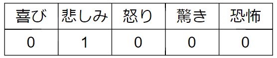
正解値の「悲しみ」は1でそれ以外は0になっているのが分かると思います
今度は、抜き出したデータに対して、分類モデルを適用します
その結果が以下の通りです

正解のラベルのように0と1だけにはならず、0~1の間をとっています。
これは、その値の確信度として考えることができます。
One-Hotエンコーディングでラベリングすることでその値かもしれない確信度をとるようにできます。