
Understanding Linear Regression using Ordinary Least Squares (OLS)
Linear Regression is one of the fundamental supervised learning algorithms in Machine Learning. Its objective is to find the best-fit line by minimizing the prediction error between the actual and predicted values.
The prediction equation is
$$
\hat{y}_i = mx_i + b
$$
where
- $m$ = Slope
- $b$ = Intercept
- $\hat{y}_i$ = Predicted value
Best-Fit Line
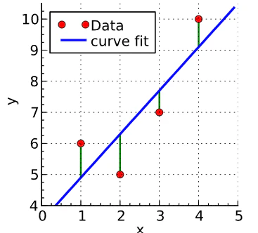
The residual (prediction error) for each data point is
$$
d_i = y_i - \hat{y}_i
$$
where
- $y_i$ = Actual target value
- $\hat{y}_i$ = Predicted target value
- $d_i$ = Residual (Prediction Error)
Error Function
The Sum of Squared Errors (SSE) is
$$
E=\sum_{i=1}^{n}d_i^2
$$
Substituting
$$
d_i=y_i-\hat{y}_i
$$
gives
$$
E=\sum_{i=1}^{n}(y_i-\hat{y}_i)^2
$$
Since
$$
\hat{y}_i=mx_i+b
$$
the error function becomes
$$
E=\sum_{i=1}^{n}(y_i-mx_i-b)^2
$$
Objective
Our objective is to find the values of $m$ and $b$ that minimize the error function.
Therefore,
$$
\frac{\partial E}{\partial m}=0
$$
and
$$
\frac{\partial E}{\partial b}=0
$$
Derivation of the Intercept (b)
Differentiate the error function with respect to $b$.
$$
\frac{\partial E}{\partial b}
$$
$$
\frac{\partial}{\partial b}
\sum_{i=1}^{n}(y_i-mx_i-b)^2
=0
$$
Applying the chain rule,
$$
\sum_{i=1}^{n}
2(y_i-mx_i-b)(-1)=0
$$
$$
-2\sum_{i=1}^{n}(y_i-mx_i-b)=0
$$
Divide both sides by $-2$.
$$
\sum_{i=1}^{n}(y_i-mx_i-b)=0
$$
Expanding,
$$
\sum_{i=1}^{n}y_i - m\sum_{i=1}^{n}x_i - \sum_{i=1}^{n}b = 0
$$
Since $b$ is a constant,
$$
\sum_{i=1}^{n}b = nb
$$
Substitute this into the equation.
$$
\sum_{i=1}^{n}y_i - m\sum_{i=1}^{n}x_i - nb = 0
$$
Now divide every term by $n$.
$$
\frac{1}{n}\sum_{i=1}^{n}y_i-
m\frac{1}{n}\sum_{i=1}^{n}x_i-
\frac{nb}{n}=
0
$$
Simplifying,
$$
\frac{1}{n}\sum_{i=1}^{n}y_i-
m\frac{1}{n}\sum_{i=1}^{n}x_i-
b=
0
$$
Using
$$
\bar{y}=\frac{1}{n}\sum_{i=1}^{n}y_i
$$
and
$$
\bar{x}=\frac{1}{n}\sum_{i=1}^{n}x_i
$$
we obtain
$$
\bar{y}-m\bar{x}-b=0
$$
Therefore,
$$
b=\bar{y}-m\bar{x}
$$
Derivation of the Slope (m)
Substitute
$$
b=\bar{y}-m\bar{x}
$$
into the error function.
$$
E=
\sum_{i=1}^{n}
(y_i-mx_i-\bar{y}+m\bar{x})^2
$$
Differentiate with respect to $m$.
$$
\frac{\partial E}{\partial m}=0
$$
$$
\sum_{i=1}^{n}
2(y_i-mx_i-\bar{y}+m\bar{x})
(-x_i+\bar{x})
=0
$$
Multiply both sides by $-1$.
$$
\sum_{i=1}^{n}
2(y_i-mx_i-\bar{y}+m\bar{x})
(x_i-\bar{x})
=0
$$
Divide both sides by $2$.
$
\sum_{i=1}^{n}
\left[
(y_i-\bar{y})-
m(x_i-\bar{x})
\right]
(x_i-\bar{x})
=0
$$
Expand the expression.
$$
\sum_{i=1}^{n}
(y_i-\bar{y})(x_i-\bar{x})-
m
\sum_{i=1}^{n}
(x_i-\bar{x})^2
=0
$$
Move the second term to the right-hand side.
$$
\sum_{i=1}^{n}
(y_i-\bar{y})(x_i-\bar{x})=
m
\sum_{i=1}^{n}
(x_i-\bar{x})^2
$$
Finally,
$$
\boxed{
m=
\frac{
\sum_{i=1}^{n}(y_i-\bar{y})(x_i-\bar{x})
}{
\sum_{i=1}^{n}(x_i-\bar{x})^2
}
}
$$
Final Linear Regression Model
The final prediction equation is
$$
\boxed{
\hat{y}=mx+b
}
$$
where
$$
\boxed{
m=
\frac{
\sum_{i=1}^{n}(y_i-\bar{y})(x_i-\bar{x})
}{
\sum_{i=1}^{n}(x_i-\bar{x})^2
}
}
$$
and
$$
\boxed{
b=\bar{y}-m\bar{x}
}
$$
Notation
| Symbol | Description |
|---|---|
| $x_i$ | Input data point |
| $y_i$ | Actual target value |
| $\hat{y}_i$ | Predicted target value |
| $d_i$ | Residual (Prediction Error) |
| $\bar{x}$ | Mean of all input values |
| $\bar{y}$ | Mean of all target values |
| $m$ | Slope |
| $b$ | Intercept |
Conclusion
In this article, we derived the closed-form solution of Simple Linear Regression using the Ordinary Least Squares (OLS) method.
By minimizing the Sum of Squared Errors (SSE), we obtained the optimal values of the slope ($m$) and intercept ($b$).
The final regression equation is
$$
\hat{y}=mx+b
$$
where
$$
m=
\frac{
\sum_{i=1}^{n}(y_i-\bar{y})(x_i-\bar{x})
}{
\sum_{i=1}^{n}(x_i-\bar{x})^2
}
,\qquad
b=\bar{y}-m\bar{x}
$$