今回は、Self-Attentionを実装してみます。Self-Attentionにより、どの時刻のデータをより重要と考えているかがわかります。
ディープラーニングを実装から学ぶ(10-1)RNNの実装(RNN,LSTM,GRU)、ディープラーニングを実装から学ぶ(10-2)RNNの実装(双方向RNN・orthogonal(重みの初期値))の続きです。
例によって、MNISTで確認していきます。
Self-Attention
Attentionは、注意機構と呼ばれ、どの時刻に注目するかを決めます。
特に今回は、自分のRNNの出力をベースに、注目する時刻を決めるため、Self-Attentionと呼ばれます。
下図のように、双方向RNNの結果を受け、注目する時刻を確率で決めます。すべての時刻の和は、1となります。
注目確率の高い時刻のデータがより利用され重要な情報であることがわかります。

(本来は、Attentionの値は、RNNの各時刻からの出力で決定されますが、簡略化して図示しています。)
スコア関数
各時刻の確率を決定するための関数がスコア関数です。いろいろなスコア関数が利用されるようですが、ここでは、以下の関数を利用します。
W_2\mathrm{tanh}(W_1hs+b_1)+b_2
通常の全結合型のaffine変換を2回行います。活性化関数は、$ \mathrm{tanh} $です。
最後に、softmax関数を通して、各時刻ごとの確率に変換します。
順伝播
Self-Attention層の順伝播を考えます。Self-Attention層は、以下の図の構造をしています。
①が、双方向RNNからの入力です。
上段(②~⑤)がスコア計算部になります。affine変換の一層目(②)のノード数(d)は、ハイパーパラメータで任意に決定します。二層目(④)のノード数は、1になります。
①に、上段で計算した確率を掛けます(⑥)。最後に、各時刻のデータを合計し最終的な出力(⑦)とします。

スコア部分の実装です。
affine、活性化関数の全結合型の実装です。一層目の活性化関数は、変更できるようにしています。二層目は、確率を求めるため、softmaxです。
1点注意点です。softmaxは、時刻に対して確率を求めるため、reshapeを行っています。
    n, t, h = u.shape
    # score計算
    # u - (n, t, h)
    # W1 - (h, d)
    # b - h2
    s1 = affine(u, W1, b1)
    # s1 - (n, t, d)
    s1z = propagation_func(s1)
    # s1z - (n, t, d)
    # W2 - (d, 1)
    # b2 - 1
    s2 = affine(s1z, W2, b2)
    # s2 - (n, t, 1)
    score = s2.reshape(n, t)
    # 各時間の確率に変換
    attention_weight = softmax(score)
双方向RNNからの入力と確率を掛け合わせて時刻ごとの値を計算します。最後にsumで全時刻の合計を求めます。
    # attention_weight - (n, t)
    z = (u * attention_weight.reshape(n, t, 1)).sum(axis=1)
関数全体です。逆伝播用に、計算途中の値を保持しておきます。
def SelfAttention(u, W1, b1, W2, b2, propagation_func=tanh):
    n, t, h = u.shape
    # score計算
    # u - (n, t, h)
    # W1 - (h, d)
    # b - h2
    s1 = affine(u, W1, b1)
    # s1 - (n, t, d)
    s1z = propagation_func(s1)
    # s1z - (n, t, d)
    # W2 - (d, 1)
    # b2 - 1
    s2 = affine(s1z, W2, b2)
    # s2 - (n, t, 1)
    score = s2.reshape(n, t)
    # 各時間の確率に変換
    attention_weight = softmax(score)
    # attention_weight - (n, t)
    z = (u * attention_weight.reshape(n, t, 1)).sum(axis=1)
    # z - (n, h)
    return z, s1, s1z, s2, attention_weight
逆伝播
逆伝播の図です。それぞれの勾配を赤字で記載しています。
逆伝播は、後ろから順に掛けていけばよいのでした。順に見ていきましょう。

⑦ sum
合計(足し算)の勾配は、1です。
dud_{ij} = dz_{j} \times 1
そのまま1を掛ければよいのですが、時刻方向に拡張します。
    # dz - (n, h)
    dud = np.ones_like(u) * dz[:,np.newaxis,:]
    # dud- (n, t, h)
⑥ $ \times $
掛け算の勾配は、それぞれ逆方向の値になります。$ u $方向は、$ att_w $、スコア計算方向は、$ u $になります。
ここでは、スコア計算方向を考えます。
$ att\_w $は、$ u $の各時刻に掛けます。よって、勾配は、逆にh方向の値をすべて加えたものになります。
datt\_w_i = dud_{i1} \times u_{i1} + dud_{i2} \times u_{i2} + ・・・ + dud_{ih} \times u_{ih}
実装です。
    # dud- (n, t, h)
    dattention_weight = (dud * u).sum(axis=2)
    # dattention_weight - (n, t)
⑤ $ \mathrm{softmax} $
softmaxの勾配は、以前求めました。ただし、実装は損失関数と合わせてsoftmax_cross_entropy_error_backとしていました。ここでは、独立して実装します。
softmaxの勾配は、以前の記事を参考にしてください。
ディープラーニングを実装から学ぶ(4-2)学習(誤差逆伝播法2) softmax関数の勾配
$ \mathrm{softmax} $の勾配は、以下になります。
softmax'(x_i) = softmax(x_i) - \sum_{k=0}^tsoftmax(x_k) \times softmax(x_i)
勾配関数の実装です。
def softmax_back(dz, u, z):
    return dz * z - np.sum(dz * z, axis=1)[:,np.newaxis] * z
$ \mathrm{softmax} $の勾配計算は、勾配関数を呼ぶだけです。その後、affine用に次元拡張しておきます。
    # dattention_weight - (n, t)
    dscore = softmax_back(dattention_weight, s2, attention_weight)
    ds2 = dscore.reshape(n, t, 1)
    # ds2 - (n, t, 1)
④ affine
affineの勾配は、実装済のaffineの勾配関数を呼ぶだけです。ただし、時系列データは、バッチサイズ、時系列長、出力次元数の3次元です。現状のaffineの勾配関数は、3次元に対応していません。一旦、2次元に変換し勾配を求め、最後に3次元に戻すように実装を変更します。
def affine_back(dz, u, W, b, calc_du_flag=True):
    dzr = dz.reshape(-1,dz.shape[-1])
    ur = u.reshape(-1,u.shape[-1])
    dur = None
    if calc_du_flag:                        # 最初の層では、duを計算しない
        dur = np.dot(dzr, W.T)                # zの勾配は、今までの勾配と重みを掛けた値
    dW = np.dot(ur.T, dzr)                    # 重みの勾配は、zに今までの勾配を掛けた値
    db = np.dot(np.ones(ur.shape[0]).T, dzr)  # バイアスの勾配は、今までの勾配の値
    du = None
    if calc_du_flag:                        # 最初の層では、duを計算しない
        du = dur.reshape(u.shape)
    return du, dW, db
勾配は、実装を変更したaffine_backを呼び出します。
    # ds2 - (n, t, 1)
    ds1z, dW2, db2 = affine_back(ds2, s1z, W2, b2)
    # ds1z - (n, t, d)
③ $ \mathrm{tanh} $
$ \mathrm{tanh} $の勾配関数を呼び出します。
実装です。ここでは、指定した関数の勾配関数を呼び出します。
    # ds1z - (n, t, d)
    ds1 = propagation_back_func(ds1z, s1, s1z)
    # ds1 - (n, t, d)
② affine
④で実装変更したaffineの勾配関数を呼び出します。
    # ds1 - (n, t, d)
    du1, dW1, db1 = affine_back(ds1, u, W1, b1)
    # du1 - (n, t, h)
① 分岐
最後に分岐の対応です。分岐は、それぞれの方向の勾配を加えます。
ここでは、スコア計算方向と$ ud $方向の両方の勾配を加えます。
    # du1 - (n, t, h)
    du = du1 + dud * attention_weight[:,:,np.newaxis]
全体の実装です。
def SelfAttention_back(dz, u, z, s1, s1z, s2, attention_weight, W1, b1, W2, b2, propagation_func=tanh):
    n, t, h = u.shape
    propagation_back_func = eval(propagation_func.__name__ + "_back")
    # dz - (n, h)
    dud = np.ones_like(u) * dz[:,np.newaxis,:]
    # dud- (n, t, h)
    dattention_weight = (dud * u).sum(axis=2)
    # dattention_weight - (n, t)
    dscore = softmax_back(dattention_weight, s2, attention_weight)
    ds2 = dscore.reshape(n, t, 1)
    # ds2 - (n, t, 1)
    ds1z, dW2, db2 = affine_back(ds2, s1z, W2, b2)
    # ds1z - (n, t, d)
    ds1 = propagation_back_func(ds1z, s1, s1z)
    # ds1 - (n, t, d)
    du1, dW1, db1 = affine_back(ds1, u, W1, b1)
    # du1 - (n, t, h)
    du = du1 + dud * attention_weight[:,:,np.newaxis]
    return du, dW1, db1, dW2, db2
フレームワーク対応
初期化時に、スコア演算の1つ目のaffine変換のノード数を与えます。2つ目のaffine変換のノード数は、1固定のため指定しません。
def SelfAttention_init_layer(d_prev, d, weight_init_func=glorot_normal, weight_init_params={}, bias_init_func=zeros_b, bias_init_params={}, **params):
    t, h = d_prev
    d_next = h
    W1 = weight_init_func(h, d, **weight_init_params)
    b1 = bias_init_func(d, **bias_init_params)
    W2 = weight_init_func(d, 1, **weight_init_params)
    b2 = bias_init_func(1, **bias_init_params)
    return d_next, {"W1":W1, "b1":b1, "W2":W2, "b2":b2}

def SelfAttention_init_optimizer():
    sW1 = {}
    sb1 = {}
    sW2 = {}
    sb2= {}
    return {"sW1":sW1, "sb1":sb1, "sW2":sW2, "sb2":sb2}

def SelfAttention_propagation(func, u, weights, weight_decay, learn_flag, propagation_func=tanh, **params):
    # SelfAttention
    z, s1, s1z, s2, attention_weight = func(u, weights["W1"], weights["b1"], weights["W2"], weights["b2"], propagation_func)
    # 重み減衰対応
    weight_decay_r = 0
    if weight_decay is not None:
        weight_decay_r += weight_decay["func"](weights["W1"], **weight_decay["params"])
        weight_decay_r += weight_decay["func"](weights["W2"], **weight_decay["params"])
    return {"u":u, "z":z, "s1":s1, "s1z":s1z, "s2":s2, "attention_weight":attention_weight}, weight_decay_r

def SelfAttention_back_propagation(back_func, dz, us, weights, weight_decay, calc_du_flag, propagation_func=tanh, **params):
    # SelfAttentionの勾配計算
    du, dW1, db1, dW2, db2 = back_func(dz, us["u"], us["z"], us["s1"], us["s1z"], us["s2"], us["attention_weight"], weights["W1"], weights["b1"], weights["W2"], weights["b2"], propagation_func)
    # 重み減衰対応
    if weight_decay is not None:
        dW1 += weight_decay["back_func"](weights["W1"], **weight_decay["params"])
        dW2 += weight_decay["back_func"](weights["W2"], **weight_decay["params"])
    return {"du":du, "dW1":dW1, "db1":db1, "dW2":dW2, "db2":db2}

def SelfAttention_update_weight(func, du, weights, optimizer_stats, **params):
    weights["W1"], optimizer_stats["sW1"] = func(weights["W1"], du["dW1"], **params, **optimizer_stats["sW1"])
    weights["b1"], optimizer_stats["sb1"] = func(weights["b1"], du["db1"], **params, **optimizer_stats["sb1"])
    weights["W2"], optimizer_stats["sW2"] = func(weights["W2"], du["dW2"], **params, **optimizer_stats["sW2"])
    weights["b2"], optimizer_stats["sb2"] = func(weights["b2"], du["db2"], **params, **optimizer_stats["sb2"])
    return weights, optimizer_stats
実行例
「ディープラーニングを実装から学ぶ(8)実装変更」の「参考」-「プログラム全体」のプログラムおよび「ディープラーニングを実装から学ぶ(10-2)RNNの実装(双方向RNN・orthogonal(重みの初期値))の「参考」-「プログラム」を事前に実行しておきます。
MNISTのデータを読み込みます。(MNISTのデータファイルが、c:\mnistに格納されている例)
x_train, t_train, x_test, t_test = load_mnist('c:\\mnist\\')
data_normalizer = create_data_normalizer(min_max)
nx_train, data_normalizer_stats = train_data_normalize(data_normalizer, x_train)
nx_test                         = test_data_normalize(data_normalizer, x_test)
時系列データとなるようにreshapeします。
nx_train = nx_train.reshape((nx_train.shape[0], 28, 28))
nx_test  = nx_test.reshape((nx_test.shape[0], 28, 28))
モデルを定義します。双方向RNNの次の層にSelfAttentionを置きます。
SelfAttentionの入力は、$ hs $のため、双方向RNNにreturn_hs=Trueを設定します。スコア計算用のノード数は、28にしました。
model = create_model((28,28))
model = add_layer(model, "BiRNN1", BiRNN, 100, merge="sum", return_hs=True)
model = add_layer(model, "SelfAttention1", SelfAttention, 28)
model = add_layer(model, "affine", affine, 10)
model = set_output(model, softmax)
model = set_error(model, cross_entropy_error)
optimizer = create_optimizer(SGD, lr=0.01)

epoch = 30
batch_size = 100
np.random.seed(10)
model, optimizer, learn_info = learn(model, nx_train, t_train, nx_test, t_test, batch_size=batch_size, epoch=epoch, optimizer=optimizer)
結果です。
input - 0 (28, 28)
BiRNN1 BiRNN (28, 28) (28, 100)
SelfAttention1 SelfAttention (28, 100) 100
affine affine 100 10
output softmax 10
error cross_entropy_error
0 0.09958333333333333 2.356261961149907 0.0968 2.3614130750977416
1 0.5678833333333333 1.3848304920746923 0.8275 0.6690278528691983
2 0.8664333333333334 0.4880185742962618 0.8874 0.39362351884719565
3 0.9151166666666667 0.30426044306014594 0.9329 0.24496483790721163
4 0.9336333333333333 0.2350918895586123 0.9384 0.21948361392290694
5 0.94355 0.19849007625957393 0.9469 0.19187446158294214
6 0.9491 0.1752445828755755 0.9541 0.1655796201180502
7 0.9547833333333333 0.15731748179078986 0.9585 0.14616701632164786
8 0.9583333333333334 0.14399193313569525 0.9587 0.14235769452023372
9 0.9621666666666666 0.13279317238922064 0.9645 0.12292895510716585
10 0.9646 0.12306893122205227 0.9662 0.11727785604947412
11 0.9666333333333333 0.11586099924548256 0.9649 0.1158738665468039
12 0.9687833333333333 0.10817244090372792 0.9702 0.10706760744361034
13 0.9699666666666666 0.10287234574974215 0.9668 0.12015481665692414
14 0.9716166666666667 0.09717223367873985 0.9718 0.10097834374159101
15 0.9730333333333333 0.0941378189965908 0.9696 0.10482215077132623
16 0.9742 0.08973221984824362 0.9717 0.09406318599207183
17 0.9761166666666666 0.08470828968398411 0.9714 0.09676668253958177
18 0.9766666666666667 0.08185968641346138 0.9739 0.09297079396236534
19 0.9770166666666666 0.07943368098198679 0.9746 0.08632488969711463
20 0.9778166666666667 0.07704190050053451 0.9734 0.09088251387408858
21 0.9786333333333334 0.07467714609974876 0.9758 0.08350655587801789
22 0.9798166666666667 0.07116746647333412 0.9767 0.08486943004984739
23 0.9803333333333333 0.06869498928688969 0.9777 0.08217006912332941
24 0.9802833333333333 0.06853395584919589 0.9774 0.07909381568395833
25 0.9820166666666666 0.06451569687728087 0.9767 0.08322501912543342
26 0.9812333333333333 0.06402819034588025 0.9773 0.07991737127583279
27 0.9822666666666666 0.06139960612790664 0.9777 0.07854774302284892
28 0.9828833333333333 0.05994977285326149 0.9761 0.08377384513462806
29 0.9833 0.05831958540478948 0.9769 0.08123826622513966
30 0.9834166666666667 0.05779614606861226 0.9773 0.07808698872646821
所要時間 = 19 分 18 秒
双方向RNNとほぼ同等の精度が得られました。
スコア確認
各時刻のスコアを確認してみます。
まず、テストデータで予測します。
y_pred, err, us = predict(model, nx_test, t_test)
スコアは、"SelfAttention1"層の"attention_weight"に格納されています。
最初のデータの値を表示してみます。
us["SelfAttention1"]["attention_weight"][0]
array([3.25055418e-05, 1.48083012e-05, 6.65611187e-06, 4.44442070e-06,
       9.71415843e-06, 8.85175022e-05, 5.19578835e-04, 2.39988947e-02,
       7.36965088e-01, 2.18292202e-01, 5.97463083e-03, 1.28431815e-03,
       6.89662842e-04, 8.56142294e-04, 8.40103802e-04, 1.88555610e-04,
       2.94774366e-05, 3.46360713e-05, 1.59697117e-04, 1.91259827e-04,
       7.67783816e-05, 7.57458645e-05, 6.07694607e-04, 4.70357651e-03,
       3.05888981e-03, 8.90751434e-04, 2.07097954e-04, 1.98571918e-04])
予想通り、ほとんど数字の含まれない上部や下部の値は確率が非常に低くなっております。中央あたりが高い値になっています。
確認のため、すべての値を合計してみます。若干誤差はありますが、1になりました。
np.sum(us["SelfAttention1"]["attention_weight"][0])
1.0000000000000002
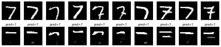
画像に確率を表示してみます。7の上の横棒部分の確率が高くなっています。

データに確率を掛けて表示してみます。ただし、確率を掛けると小さな値となるため、28倍しました。
nx_test[0]*us["SelfAttention1"]["attention_weight"][0].reshape(-1,1)*28
表示してみます。

このように見えているのですかね。
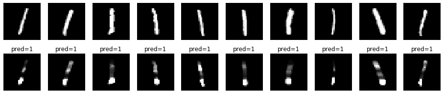
先頭から10画像分について確認してみます。
上が元の画像、下が確率を掛けた画像です。特徴的な位置を捉えているようにも見えます。

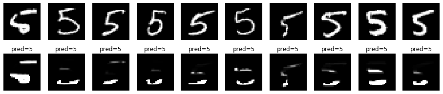
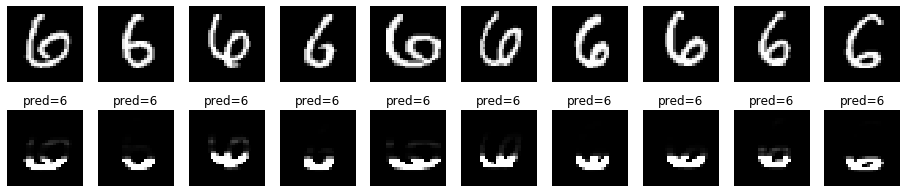
数字ごとに違いがあるか、各数字について先頭から10画像分確認してみます。
0

1
2

3

4

5
6
7
8

9

どうでしょう。
数字の特徴的な部分を捉えているのでしょうか?
数字ごとに確率が高いところが異なります。
参考
SelfAttentionおよび今回変更したプログラムです。
関数仕様
# 層追加関数
model = add_layer(model, name, func, d=None, **kwargs)
# 引数
#  model : モデル
#  name  : レイヤの名前
#  func  : 中間層の関数
#           affine,sigmoid,tanh,relu,leaky_relu,prelu,rrelu,relun,srelu,elu,maxout,
#           identity,softplus,softsign,step,dropout,batch_normalization,
#           convolution2d,max_pooling2d,average_pooling2d,flatten2d,
#           RNN,LSTM,GRU,BiRNN, BiLSTM,BiGRU, SelfAttention
#  d     : ノード数
#           affine,maxout,convolution2d,RNN,LSTM,GRU,BiRNN, BiLSTM,BiGRUの場合指定
#           convolution2dの場合は、フィルタ数
#           RNN,LSTM,GRU,BiRNN, BiLSTM,BiGRUの場合は、出力次元数
#  kwargs: 中間層の関数のパラメータ
#           affine - weight_init_func=he_normal, weight_init_params={}, bias_init_func=zeros_b, bias_init_params={}
#                     weight_init_func - lecun_normal,lecun_uniform,glorot_normal,glorot_uniform,he_normal,he_uniform,normal_w,uniform_w,zeros_w,ones_w
#                     weight_init_params
#                       normal_w - mean=0, var=1
#                       uniform_w - min=0, max=1
#                     bias_init_func - normal_b,uniform_b,zeros_b,ones_b
#                     bias_init_params
#                       normal_b - mean=0, var=1
#                       uniform_b - min=0, max=1
#           leaky_relu - alpha
#           rrelu - min=0.0, max=0.1
#           relun - n
#           srelu - alpha
#           elu - alpha
#           maxout - unit=1, weight_init_func=he_normal, weight_init_params={}, bias_init_func=zeros_b, bias_init_params={}
#           dropout - dropout_ratio=0.9
#           batch_normalization - batch_norm_node=True, use_gamma_beta=True, use_train_stats=True, alpha=0.1
#           convolution2d - padding=0, strides=1, weight_init_func=he_normal, weight_init_params={}, bias_init_func=zeros_b, bias_init_params={}
#           max_pooling2d - pool_size=2, padding=0, strides=None
#           average_pooling2d - pool_size=2, padding=0, strides=None
#           RNN, LSTM, GRU - propagation_func=tanh, return_hs=False, Wx_init_func=glorot_normal, Wx_init_params={}, Wh_init_func=glorot_normal, Wh_init_params={}, bias_init_func=zeros_b, bias_init_params={}
#                            propagation_func - tanh,sigmoid,relu
#                            Wx_init_func, Wh_init_funcは、affineのweight_init_funcに同じ。Wh_init_funcは、orthogonalも指定可能
#           BiRNN, BiLSTM, BiGRU - propagation_func=tanh, return_hs=False, merge="concat", input_dictionary=False, Wx_init_func=glorot_normal, Wx_init_params={}, Wh_init_func=glorot_normal, Wh_init_params={}, bias_init_func=zeros_b, bias_init_params={}
#                                  propagation_func - tanh,sigmoid,relu
#                                  merge - "concat", "sum", "dictionary"
#                                  Wx_init_func, Wh_init_funcは、affineのweight_init_funcに同じ。Wh_init_funcは、orthogonalも指定可能
#           SelfAttention - propagation_func=tanh, weight_init_func=glorot_normal, weight_init_params={}, bias_init_func=zeros_b, bias_init_params={}
# 戻り値
#  モデル
プログラム
# affine変換
def affine(u, W, b):
    return np.dot(u, W) + b

def affine_back(dz, u, W, b, calc_du_flag=True):
    dzr = dz.reshape(-1,dz.shape[-1])
    ur = u.reshape(-1,u.shape[-1])
    dur = None
    if calc_du_flag:                        # 最初の層では、duを計算しない
        dur = np.dot(dzr, W.T)                # zの勾配は、今までの勾配と重みを掛けた値
    dW = np.dot(ur.T, dzr)                    # 重みの勾配は、zに今までの勾配を掛けた値
    db = np.dot(np.ones(ur.shape[0]).T, dzr)  # バイアスの勾配は、今までの勾配の値
    du = None
    if calc_du_flag:                        # 最初の層では、duを計算しない
        du = dur.reshape(u.shape)
    return du, dW, db

def softmax(u):
    u = u.T
    max_u = np.max(u, axis=0)
    exp_u = np.exp(u - max_u)
    sum_exp_u = np.sum(exp_u, axis=0)
    y = exp_u/sum_exp_u
    return y.T

def softmax_back(dz, u, z):
    return dz * z - np.sum(dz * z, axis=1)[:,np.newaxis] * z
def SelfAttention(u, W1, b1, W2, b2, propagation_func=tanh):
    n, t, h = u.shape
    # score計算
    # u - (n, t, h)
    # W1 - (h, d)
    # b - h2
    s1 = affine(u, W1, b1)
    # s1 - (n, t, d)
    s1z = propagation_func(s1)
    # s1z - (n, t, d)
    # W2 - (d, 1)
    # b2 - 1
    s2 = affine(s1z, W2, b2)
    # s2 - (n, t, 1)
    score = s2.reshape(n, t)
    # 各時間の確率に変換
    attention_weight = softmax(score)
    # attention_weight - (n, t)
    z = (u * attention_weight.reshape(n, t, 1)).sum(axis=1)
    # z - (n, h)
    return z, s1, s1z, s2, attention_weight

def SelfAttention_back(dz, u, z, s1, s1z, s2, attention_weight, W1, b1, W2, b2, propagation_func=tanh):
    n, t, h = u.shape
    propagation_back_func = eval(propagation_func.__name__ + "_back")
    # dz - (n, h)
    dud = np.ones_like(u) * dz[:,np.newaxis,:]
    # dud- (n, t, h)
    dattention_weight = (dud * u).sum(axis=2)
    # dattention_weight - (n, t)
    dscore = softmax_back(dattention_weight, s2, attention_weight)
    ds2 = dscore.reshape(n, t, 1)
    # ds2 - (n, t, 1)
    ds1z, dW2, db2 = affine_back(ds2, s1z, W2, b2)
    # ds1z - (n, t, d)
    ds1 = propagation_back_func(ds1z, s1, s1z)
    # ds1 - (n, t, d)
    du1, dW1, db1 = affine_back(ds1, u, W1, b1)
    # du1 - (n, t, h)
    du = du1 + dud * attention_weight[:,:,np.newaxis]
    return du, dW1, db1, dW2, db2
def SelfAttention_init_layer(d_prev, d, weight_init_func=glorot_normal, weight_init_params={}, bias_init_func=zeros_b, bias_init_params={}, **params):
    t, h = d_prev
    d_next = h
    W1 = weight_init_func(h, d, **weight_init_params)
    b1 = bias_init_func(d, **bias_init_params)
    W2 = weight_init_func(d, 1, **weight_init_params)
    b2 = bias_init_func(1, **bias_init_params)
    return d_next, {"W1":W1, "b1":b1, "W2":W2, "b2":b2}

def SelfAttention_init_optimizer():
    sW1 = {}
    sb1 = {}
    sW2 = {}
    sb2= {}
    return {"sW1":sW1, "sb1":sb1, "sW2":sW2, "sb2":sb2}

def SelfAttention_propagation(func, u, weights, weight_decay, learn_flag, propagation_func=tanh, **params):
    # SelfAttention
    z, s1, s1z, s2, attention_weight = func(u, weights["W1"], weights["b1"], weights["W2"], weights["b2"], propagation_func)
    # 重み減衰対応
    weight_decay_r = 0
    if weight_decay is not None:
        weight_decay_r += weight_decay["func"](weights["W1"], **weight_decay["params"])
        weight_decay_r += weight_decay["func"](weights["W2"], **weight_decay["params"])
    return {"u":u, "z":z, "s1":s1, "s1z":s1z, "s2":s2, "attention_weight":attention_weight}, weight_decay_r

def SelfAttention_back_propagation(back_func, dz, us, weights, weight_decay, calc_du_flag, propagation_func=tanh, **params):
    # SelfAttentionの勾配計算
    du, dW1, db1, dW2, db2 = back_func(dz, us["u"], us["z"], us["s1"], us["s1z"], us["s2"], us["attention_weight"], weights["W1"], weights["b1"], weights["W2"], weights["b2"], propagation_func)
    # 重み減衰対応
    if weight_decay is not None:
        dW1 += weight_decay["back_func"](weights["W1"], **weight_decay["params"])
        dW2 += weight_decay["back_func"](weights["W2"], **weight_decay["params"])
    return {"du":du, "dW1":dW1, "db1":db1, "dW2":dW2, "db2":db2}

def SelfAttention_update_weight(func, du, weights, optimizer_stats, **params):
    weights["W1"], optimizer_stats["sW1"] = func(weights["W1"], du["dW1"], **params, **optimizer_stats["sW1"])
    weights["b1"], optimizer_stats["sb1"] = func(weights["b1"], du["db1"], **params, **optimizer_stats["sb1"])
    weights["W2"], optimizer_stats["sW2"] = func(weights["W2"], du["dW2"], **params, **optimizer_stats["sW2"])
    weights["b2"], optimizer_stats["sb2"] = func(weights["b2"], du["db2"], **params, **optimizer_stats["sb2"])
    return weights, optimizer_stats