概要
既にQiita上で試している方もいらっしゃいましたが、自身の勉強も兼ねて
CNN(ResNet)を使ってギター画像の分類をやってみたのでその過程で試したこと、
参考になりそうなことを紹介します。(まとめていないので若干汚いですがコードも載せていきます)
目次
- 具体的な分類方法
- 前処理について
- 学習方法について
- 学習結果について
- 試して遊んでみる
- まとめ
具体的な分類方法について
ギター画像をスクレイピングにより取得し、それに前処理を施して画像を水増しします。
水増しした画像を用いてCNNの一手法であるResNetをファインチューニングさせることで、
学習コストをあまりかけずに機械学習させてみようと思います。
ラベルについて
画像の収集が比較的簡単そうな以下の機種を選びました。
- Fender製
- ストラトキャスター
- テレキャスター
- ジャズマスター
- ジャガー
- ムスタング(含む類似機種)
- Gibson製
- レスポール
- SG
- ES-335
- フライングV
- その他
- アコースティックギター各種
前処理について
まずは画像を収集するところからです。今回はiCrawlerを用いて収集しました。
一般的にはGoogle画像検索から収集するものが多いですが、2020/3/12現在、Google側の仕様変更により
ツールが機能しなくなっているようなので今回はBingから画像を収集しました。
import os

from icrawler.builtin import BingImageCrawler

searching_words = [
                    "Fender Stratocaster",
                    "Fender Telecaster",
                    "Fender Jazzmaster",
                    "Fender Jaguar",
                    "Fender Mustang",
                    "Gibson LesPaul",
                    "Gibson SG",
                    "Gibson FlyingV",
                    "Gibson ES-335",
                    "Acoustic guitar"
                ]
if __name__ == "__main__":
    for word in searching_words:
        if not os.path.isdir('./searched_image/' + word):
            os.makedirs('./searched_image/' + word)
        bing_crawler = BingImageCrawler(storage={ 'root_dir': './searched_image/' + word })
        bing_crawler.crawl(keyword=word, max_num=1000)
収集した後は、使えそうにない画像(ギター全身が写っていないもの、文字が入っているもの、手などの映り込みがあるもの等)を手動で省きました。
その結果、各ラベルごとに100~160枚程度の画像を集めることができました。(crawlメソッドにmax_num=1000を指定しましたが、400枚程度しか集めてきてくれませんでした)
続いて、収集した画像に前処理を施していきます。今回は45°ずつ画像を回転させ、反転させる処理を施しました。なので結果は16倍に増えて各ラベルごとに1600枚~2000枚程度の画像になりました。
import os
import glob

from PIL import Image
import numpy as np
from sklearn.model_selection import train_test_split

# 圧縮する画像のサイズ
image_size = 224
# トレーニングデータの数
traindata = 1000
# テストデータの数
testdata = 300

# 入力フォルダ名
src_dir = './searched_image'
# 出力フォルダ名
dst_dir = './input_guitar_data'

# 識別するラベル名
labels = [
                    "Fender Stratocaster",
                    "Fender Telecaster",
                    "Fender Jazzmaster",
                    "Fender Jaguar",
                    "Fender Mustang",
                    "Gibson LesPaul",
                    "Gibson SG",
                    "Gibson FlyingV",
                    "Gibson ES-335",
                    "Acoustic guitar"
                ]
# 画像の読み込み
for index, label in enumerate(labels):
    files =glob.glob("{}/{}/all/*.jpg".format(src_dir, label))

    #画像を変換したデータ
    X = []
    #ラベル
    Y = []

    for file in files:
        #画像を開く
        img = Image.open(file)
        img = img.convert("RGB")

        #===================#正方形に変換する#===================#
        width, height = img.size
        #縦長なら横に拡張する
        if width < height:
            result = Image.new(img.mode,(height, height),(255, 255, 255))
            result.paste(img, ((height - width) // 2, 0))
        #横長なら縦に拡張する
        elif width > height:
            result = Image.new(img.mode,(width, width),(255, 255, 255))
            result.paste(img, (0, (width - height) // 2))
        else:
            result = img

        #画像サイズを224x224にそろえる
        result.resize((image_size, image_size))

        data = np.asarray(result)
        X.append(data)
        Y.append(index)

        #===================#データの水増し#===================#
        for angle in range(0, 360, 45):
            #回転
            img_r = result.rotate(angle)
            data = np.asarray(img_r)
            X.append(data)
            Y.append(index)

            #反転
            img_t = img_r.transpose(Image.FLIP_LEFT_RIGHT)
            data = np.asarray(img_t)
            X.append(data)
            Y.append(index)

    #正規化(0~255->0~1)
    X = np.array(X,dtype='float32') / 255.0
    Y = np.array(Y)


    #交差検証用にデータを分割する
    X_train, X_test, y_train, y_test = train_test_split(X, Y, test_size=testdata, train_size=traindata)
    xy = (X_train, X_test, y_train, y_test)
    np.save("{}/{}_{}.npy".format(dst_dir, label, index), xy)
前処理した結果を各ラベルごとにnpyファイルに保存しておきます。
学習方法について
今回はCNNの代表的な手法 ResNetを使って学習させてみようと思います。
所有してるPCにNVIDIA製GPUがついていないことから、このまま学習させようとするとCPUのみでの計算となり膨大な時間がかかるため,Google Colabを使用したGPGPU環境で以下のコードを実行・学習をさせました。(Colabの使い方,ファイルのアップロード方法等については省略します)
import gc

import keras
from keras.applications.resnet50 import ResNet50
from keras.models import Sequential, Model
from keras.layers import Conv2D, MaxPooling2D
from keras.layers import Activation, Dropout, Flatten, Dense, Input
from keras.callbacks import EarlyStopping
from keras.utils import np_utils
from keras import optimizers

from sklearn.metrics import confusion_matrix

import numpy as np
import matplotlib.pyplot as plt

# クラスラベルの定義
classes = [
                   "Fender Stratocaster",
                   "Fender Telecaster",
                   "Fender Jazzmaster",
                   "Fender Jaguar",
                   "Fender Mustang",
                   "Gibson LesPaul",
                   "Gibson SG",
                   "Gibson FlyingV",
                   "Gibson ES-335",
                   "Acoustic guitar"
               ]
num_classes = len(classes)

# 読み込む画像のサイズ
ScaleTo = 224

# メイン関数の定義
def main():
   #学習データの読み込み
   src_dir = '/content/drive/My Drive/機械学習/input_guitar_data'

   train_Xs = []
   test_Xs = []
   train_ys = []
   test_ys = []

   for index, class_name in enumerate(classes):
       file = "{}/{}_{}.npy".format(src_dir, class_name, index)
       #個別の学習ファイルを持ってくる
       train_X, test_X, train_y, test_y = np.load(file, allow_pickle=True)

       #データをひとつにまとめる
       train_Xs.append(train_X)
       test_Xs.append(test_X)
       train_ys.append(train_y)
       test_ys.append(test_y)

   #まとめたデータを結合する
   X_train = np.concatenate(train_Xs, 0)
   X_test = np.concatenate(test_Xs, 0)
   y_train = np.concatenate(train_ys, 0)
   y_test = np.concatenate(test_ys, 0)

   #ラベル付けする
   y_train = np_utils.to_categorical(y_train, num_classes)
   y_test = np_utils.to_categorical(y_test, num_classes)


   #機械学習モデルの生成
   model, history = model_train(X_train, y_train, X_test, y_test)
   model_eval(model, X_test, y_test)
   #学習の履歴を表示させる
   model_visualization(history)

def model_train(X_train, y_train, X_test, y_test):
   # ResNet50のロード。全結合層は不要なので include_top=False
   input_tensor = Input(shape=(ScaleTo, ScaleTo, 3))
   resnet50 = ResNet50(include_top=False, weights='imagenet', input_tensor=input_tensor)

   # 全結合層の作成
   top_model = Sequential()
   top_model.add(Flatten(input_shape=resnet50.output_shape[1:]))
   top_model.add(Dense(256, activation='relu'))
   top_model.add(Dropout(0.5))
   top_model.add(Dense(num_classes, activation='softmax'))

   # ResNet50と全結合層を結合してモデルを作成
   resnet50_model = Model(input=resnet50.input, output=top_model(resnet50.output))

   """
   #ResNet50の一部の重みを固定
   for layer in resnet50_model.layers[:100]:
       layer.trainable = False
   """

   # 多クラス分類を指定
   resnet50_model.compile(loss='categorical_crossentropy',
           optimizer=optimizers.SGD(lr=1e-3, momentum=0.9),
           metrics=['accuracy'])
   resnet50_model.summary()

   #学習の実行
   early_stopping = EarlyStopping(monitor='val_loss', patience=0, verbose=1)
   history = resnet50_model.fit(X_train, y_train,
                       batch_size=75,
                       epochs=25, validation_data=(X_test, y_test),
                       callbacks=[early_stopping])
   #モデルの保存
   resnet50_model.save("/content/drive/My Drive/機械学習/guitar_cnn_resnet50.h5")

   return resnet50_model, history

def model_eval(model, X_test, y_test):
   scores = model.evaluate(X_test, y_test, verbose=1)
   print("test Loss", scores[0])
   print("test Accuracy", scores[1])
   #混同行列の算出
   predict_classes = model.predict(X_test)
   predict_classes = np.argmax(predict_classes, 1)
   true_classes = np.argmax(y_test, 1)
   print(predict_classes)
   print(true_classes)
   cmx = confusion_matrix(true_classes, predict_classes)
   print(cmx)
   #推論が終わったらモデルを消去する
   del model
   keras.backend.clear_session() # ←これです
   gc.collect()

def model_visualization(history):
   # 損失値をグラフ表示
   plt.plot(history.history['loss'])
   plt.plot(history.history['val_loss'])
   plt.title('model loss')
   plt.ylabel('loss')
   plt.xlabel('epoch')
   plt.legend(['train', 'test'], loc='upper left')
   plt.show()

   # 正解率をグラフ表示
   plt.plot(history.history['acc'])
   plt.plot(history.history['val_acc'])
   plt.title('model accuracy')
   plt.ylabel('accuracy')
   plt.xlabel('epoch')
   plt.legend(['train', 'test'], loc='upper left')
   plt.show()

if __name__ == "__main__":
   main()
今回は重みを固定させないほうがval acc等の結果がよかったため、各レイヤの重みも再度学習させています。
コード上では100エポック分学習させていますが、実際にはEarly Stoppingにより実際には5エポック目で学習が終了しました。
学習結果について
結果は以下の通りになりました。
test Loss 0.09369107168481061
test Accuracy 0.9744
混同行列も出しておきます。
[[199   0   1   0   0   0   0   0   0   0]
 [  0 200   0   0   0   0   0   0   0   0]
 [  2   5 191   2   0   0   0   0   0   0]
 [  1   0  11 180   6   0   2   0   0   0]
 [  0   2   0   0 198   0   0   0   0   0]
 [  0   0   0   0   0 288   4   0   6   2]
 [  0   2   0   0   0   0 296   0   2   0]
 [  0   0   0   0   0   0   0 300   0   0]
 [  0   0   0   0   0   0   0   0 300   0]
 [  0   0   0   0   0   0   0   1   0 299]]
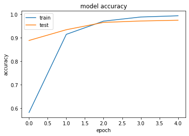
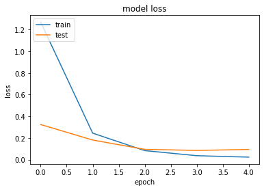
1エポック終了の時点でかなり学習が進んでいることがわかります。
試して遊んでみる
保存したモデルを基に推論を試してみようと思います。今回は初めて触ったFlaskを使って非常に初歩的なWebアプリケーションにしてみました。
import matplotlib.pyplot as plt
from PIL import Image
import numpy as np

def to_graph(image, labels, predicted):
    #=======#プロットして保存する#=======#
    fig = plt.figure(figsize=(10.24, 5.12))
    fig.subplots_adjust(left=0.2)

    #=======#横棒グラフを書く#=======#
    ax1 = fig.add_subplot(1,2,1)
    ax1.barh(labels, predicted, color='c', align="center")
    ax1.set_yticks(labels)#y軸のラベル
    ax1.set_xticks([])#x軸のラベルを消す

    # 棒グラフ内に数値を書く
    for interval, value in zip(range(0,len(labels)), predicted):
        ax1.text(0.02, interval, value, ha='left', va='center')

    #=======#判別した画像を入れる#=======#
    ax2 = fig.add_subplot(1,2,2)
    ax2.imshow(image)
    ax2.axis('off')

    return fig

def expand_to_square(input_file):
    """長方形の画像を正方形に変換する
    input_file: 変換するファイル名
    返り値:     変換された画像
    """
    img = Image.open(input_file)
    img = img.convert("RGB")

    width, height = img.size
    #縦長なら横に拡張する
    if width < height:
        result = Image.new(img.mode,(height, height),(255, 255, 255))
        result.paste(img, ((height - width) // 2, 0))
    #横長なら縦に拡張する
    elif width > height:
        result = Image.new(img.mode,(width, width),(255, 255, 255))
        result.paste(img, (0, (width - height) // 2))
    else:
        result = img

    return result
predict_file.py
import io
import gc

from flask import Flask, request, redirect, url_for
from flask import flash, render_template, make_response

from keras.models import Sequential, load_model
from keras.applications.resnet50 import decode_predictions
import keras

import numpy as np
from PIL import Image
from matplotlib.backends.backend_agg import FigureCanvasAgg

import graphing

classes = [
            "Fender Stratocaster",
            "Fender Telecaster",
            "Fender Jazzmaster",
            "Fender Jaguar",
            "Fender Mustang",
            "Gibson LesPaul",
            "Gibson SG",
            "Gibson FlyingV",
            "Gibson ES-335",
            "Acoustic guitar"
            ]
num_classes = len(classes)
image_size = 224
ALLOWED_EXTENSIONS = set(['png', 'jpg', 'gif'])


app = Flask(__name__)

def allowed_file(filename):
    return '.' in filename and filename.rsplit('.',1)[1].lower() in ALLOWED_EXTENSIONS

@app.route('/', methods=['GET', 'POST'])
def upload_file():
    if request.method == 'POST':
        if 'file' not in request.files:
            flash('ファイルがありません')
            return redirect(request.url)
        file = request.files['file']

        if file.filename == '':
            flash('ファイルがありません')
            return redirect(request.url)

        if file and allowed_file(file.filename):
            virtual_output = io.BytesIO()
            file.save(virtual_output)
            filepath = virtual_output

            model = load_model('./cnn_model/guitar_cnn_resnet50.h5')

            #画像を正方形に変換する
            image = graphing.expand_to_square(filepath)
            image = image.convert('RGB')
            #画像サイズを224x224にそろえる
            image = image.resize((image_size, image_size))
            #画像からnumpy配列に変更し正規化を行う
            data = np.asarray(image) / 255.0
            #配列の次元を増やす(3次元->4次元)
            data = np.expand_dims(data, axis=0)
            #学習したモデルを使って推論をする
            result = model.predict(data)[0]

            #推論結果と推論した画像をグラフで描画する
            fig = graphing.to_graph(image, classes, result)
            canvas = FigureCanvasAgg(fig)
            png_output = io.BytesIO()
            canvas.print_png(png_output)
            data = png_output.getvalue()

            response = make_response(data)
            response.headers['Content-Type'] = 'image/png'
            response.headers['Content-Length'] = len(data)

            #推論が終わったらモデルを消去する
            del model
            keras.backend.clear_session()
            gc.collect()

            return response
    return '''
    <!doctype html>
    <html>
        <head>
            <meta charset="UTF-8">
            <title>ファイルをアップロードして判定しよう</title>
        </head>
        <body>
            <h1>ファイルをアップロードして判定しよう!</h1>
            <form method = post enctype = multipart/form-data>
                <p><input type=file name=file>
                <input type=submit value=Upload>
            </form>
        </body>
    </html>
    '''
ちなみになのですが、Keras上で学習や推論を何回も繰り返すとメモリ上にデータが溢れてしまうようで、コード上で明示的に消去してやらないといけないようです。(colab上でも同様のようです)
参考URL↓
kerasで繰り返し学習するとメモリ使用量が増えちゃう問題を対策した
あと、実際に作ってみたウェブアプリのソースコードを載せておきます。↓
ギター分類ウェブアプリ
試して遊んでみる
所有している楽器で実際に試してみました。
まずはジャズマスターから
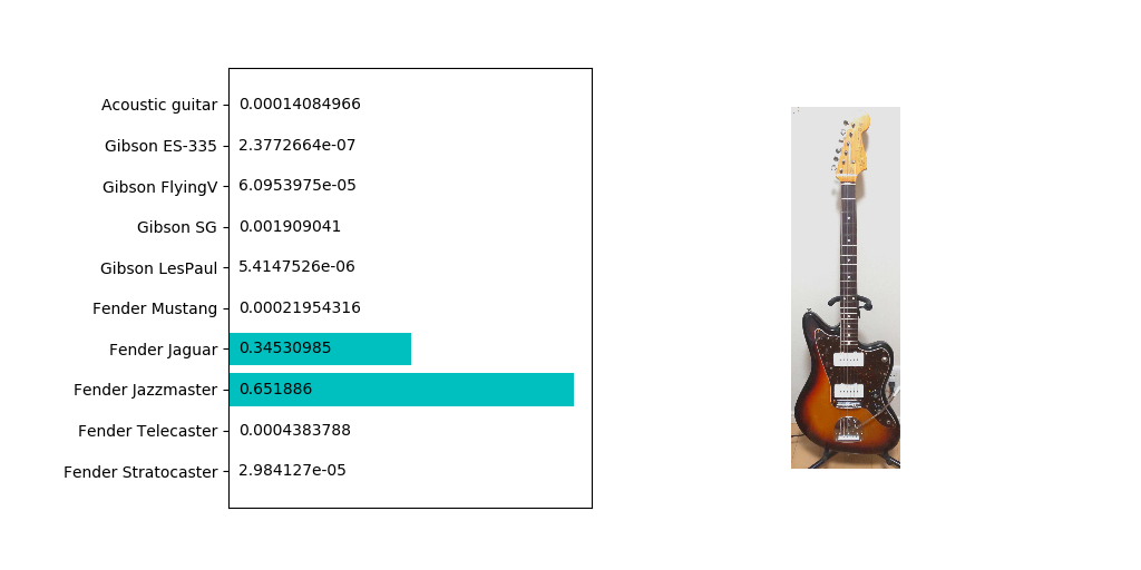
やはり類似しているところの多いジャガーにも反応していますね。
ただ他のネットから入手したほかの画像だと99%ジャズマスターだと判定されることもあるので一概に分類精度が悪いとは言えないでしょう。
続いてストラトキャスター
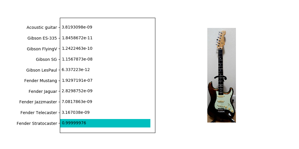
こちらはほぼ確実にストラトキャスターであることが判定されました。若干コントラストが暗めでも特に問題はないようですね。
では学習させていないベースを判定させるとどうなるでしょうか。手持ちのジャズベースタイプで試してみました。
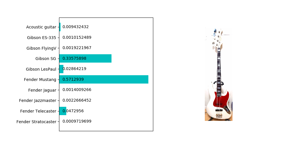
ムスタングと判定されることはわからなくもないのですが、SGの確率もそれなりに高い点であることが気になります。ツノの部分が似てなくもないような…?
まとめ
今回はCNNの一手法であるResNetをファインチューニングさせることにより、比較的作成が容易ながらも精度の高い分類器を作ることができました。
しかしながら、CNNなどの一部の機械学習はなぜ結果がそうなったのか説明し難い点は拭えません。
そこで時間があればGrad-CAMなどの可視化手法を今後は試そうと思います。
以上です。