今回は昨夜の続きです。
とにかく、機械学習~DeepLearningが何者かを理解するために、連続して画像識別をやっていきます。
その第二夜はDeepLearning界隈でたぶん一番有名なmnistの識別を機械学習、すなわち昨夜のPCA+SVCでやってみます。
そして、MLP及びDeepLearningによる識別を実施して精度などを比較することとする。
とりあえずの目標
・lfw_people.dataの識別とデータについて
・PCA+SVCによるmnistデータの識別
・MLPによるmnistの識別(・scikit-learn&keras)
・VGG16like(conv2dモデル)によるmnistの識別
・PCA+SVCによるmnistデータの識別
この後、MLPやDeepLearningの精度や時間と比較したいので、mnistデータで昨夜と同じことをやってみようと思います。
データは、昨夜も示しましたが、sklearn.datasets.fetch_openmlを利用して以下のように使えるようになったようです。
from sklearn.datasets import fetch_openml
# Load data from https://www.openml.org/d/554
X, y = fetch_openml('mnist_784', version=1, return_X_y=True)

random_state = check_random_state(0)
permutation = random_state.permutation(X.shape[0])
X = X[permutation]
y = y[permutation]
X = X.reshape((X.shape[0], -1))
X_train, X_test, y_train, y_test = train_test_split(
    X, y, train_size=train_samples, test_size=10000)
※しかし、以下のような注意書きがあり、ウワンの環境(scikit-learn v0.19)では使えませんでした
Note: EXPERIMENTAL
The API is experimental in version 0.20 (particularly the return value structure), and might have small backward-incompatible changes in future releases.
ということもあり、今回は使い慣れたKerasを使いました。
import keras
from keras.datasets import mnist
from sklearn.preprocessing import StandardScaler

train_samples=50000
n_classes=10
h,w=28,28
# the data, split between train and test sets
(x_train, y_train), (x_test, y_test) = mnist.load_data()
これを利用すると、コードは以下のとおりになります。
x_train = x_train.reshape(60000, 784)
x_train =x_train[:train_samples,:]  #data数変更用に入れました
y_train =y_train[:train_samples]    #data数変更用に入れました
x_test = x_test.reshape(10000, 784)
X_train = x_train.astype('float32')
X_test = x_test.astype('float32')
X_train /= 255
X_test /= 255

# convert class vectors to binary class matrices
scaler = StandardScaler()
X_train = scaler.fit_transform(X_train)
X_test = scaler.transform(X_test)
このデータを使うと、この後は全て前回の顔識別と同一のコードで動きました。
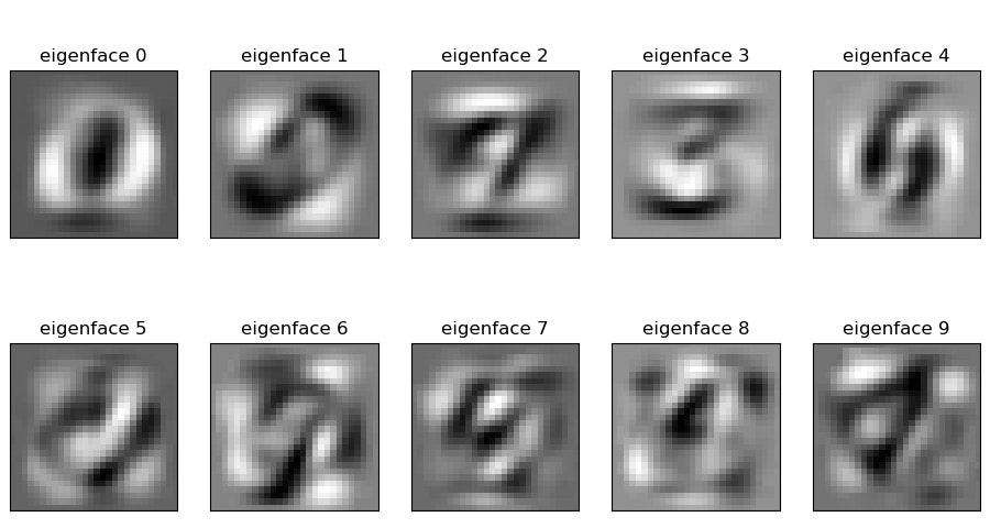
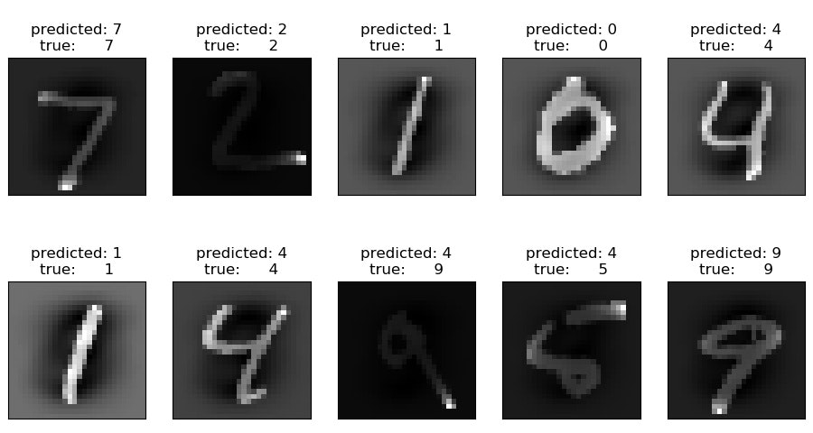
結果は、例えばtrain_samples=20000で、n_components=10とすると以下のような結果が得られました。

1599.562sもかかりました。
しかし、精度は92%程度出ています。そして、推論は1s程度と速いです。
>PYTHON peaple_pca_svc.py
None
Using TensorFlow backend.
20000 train samples
10000 test samples
Extracting the top 10 eigenfaces from 20000 faces
done in 0.351s
Projecting the input data on the eigenfaces orthonormal basis
done in 0.071s
Fitting the classifier to the training set
done in 1599.562s
Best estimator found by grid search:
SVC(C=5000.0, cache_size=200, class_weight='balanced', coef0=0.0,
  decision_function_shape='ovr', degree=3, gamma=0.01, kernel='rbf',
  max_iter=-1, probability=False, random_state=None, shrinking=True,
  tol=0.001, verbose=False)
Predicting people's names on the test set
done in 1.022s
             precision    recall  f1-score   support

          0       0.94      0.96      0.95       980
          1       0.97      0.99      0.98      1135
          2       0.93      0.93      0.93      1032
          3       0.91      0.91      0.91      1010
          4       0.90      0.90      0.90       982
          5       0.89      0.88      0.89       892
          6       0.96      0.94      0.95       958
          7       0.93      0.92      0.92      1028
          8       0.89      0.87      0.88       974
          9       0.88      0.88      0.88      1009

avg / total       0.92      0.92      0.92     10000

[[ 941    0    3    4    0   13   10    2    5    2]
 [   0 1122    1    4    1    3    2    1    1    0]
 [   8    3  963   16   11    4    4    7   16    0]
 [   1    6   18  919    1   13    0   11   34    7]
 [   4    1    6    1  887   11   10    6    5   51]
 [  19    2    3   31    9  789    6    1   27    5]
 [  18    3    8    3    8   12  901    2    1    2]
 [   0   11   16    7   10    1    0  941    3   39]
 [  11    2   18   15   14   33    7    9  849   16]
 [   3    6    4   13   44   10    1   30   13  885]]
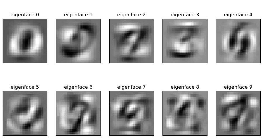
train_samples=10000で、n_components=10だと以下のとおりで、432.404sで終了しています。こちらも精度が90%程度、推論時間も0.7s弱と速いです。
>PYTHON peaple_pca_svc.py
None
Using TensorFlow backend.
10000 train samples
10000 test samples
Extracting the top 10 eigenfaces from 10000 faces
done in 0.160s
Projecting the input data on the eigenfaces orthonormal basis
done in 0.062s
Fitting the classifier to the training set
done in 432.404s
Best estimator found by grid search:
SVC(C=1000.0, cache_size=200, class_weight='balanced', coef0=0.0,
  decision_function_shape='ovr', degree=3, gamma=0.005, kernel='rbf',
  max_iter=-1, probability=False, random_state=None, shrinking=True,
  tol=0.001, verbose=False)
Predicting people's names on the test set
done in 0.686s
             precision    recall  f1-score   support

          0       0.93      0.96      0.94       980
          1       0.96      0.98      0.97      1135
          2       0.92      0.93      0.92      1032
          3       0.90      0.90      0.90      1010
          4       0.87      0.88      0.88       982
          5       0.88      0.87      0.88       892
          6       0.94      0.94      0.94       958
          7       0.92      0.90      0.91      1028
          8       0.87      0.84      0.86       974
          9       0.84      0.84      0.84      1009

avg / total       0.90      0.91      0.90     10000

[[ 936    0    3    4    0   18   12    1    5    1]
 [   0 1116    4    4    2    1    5    0    3    0]
 [   7    1  960   18    7    5    4    7   23    0]
 [   0   10   24  909    3   17    0   12   32    3]
 [   0    1    4    0  867   10   18    6    6   70]
 [  25    2    1   30   12  777    8    1   27    9]
 [  22    4   12    0    6   14  898    0    2    0]
 [   2   13   20    5    6    1    0  922    5   54]
 [  10    4   14   28   23   33    9    8  816   29]
 [   6    7    3   15   65    7    1   41   14  850]]
・MLPによるmnistの識別(・scikit-learn&keras)
次にMLPによる識別をやってみます。
その前に、MNIST classfification using multinomial logistic + L1を実施して、その後scikit-learn.MLPClassifierで識別してみます。
今回は、コードを示しつつ解説します。
import time
import matplotlib.pyplot as plt
import numpy as np
import keras
from keras.datasets import mnist
from sklearn.linear_model import LogisticRegression
from sklearn.model_selection import train_test_split
from sklearn.preprocessing import StandardScaler
from sklearn.utils import check_random_state
今回もデータはKerasのものを使います。
print(__doc__)
# Author: Arthur Mensch <arthur.mensch@m4x.org>
# License: BSD 3 clause
# Turn down for faster convergence
t0 = time.time()
train_samples = 50000
batch_size = 128
num_classes = 10
epochs = 20
# the data, split between train and test sets
(x_train, y_train), (x_test, y_test) = mnist.load_data()
x_train = x_train.reshape(60000, 784)
x_train =x_train[:train_samples,:]
y_train =y_train[:train_samples]
x_test = x_test.reshape(10000, 784)
X_train = x_train.astype('float32')
X_test = x_test.astype('float32')
X_train /= 255
X_test /= 255
scaler = StandardScaler()
X_train = scaler.fit_transform(X_train)
X_test = scaler.transform(X_test)
LogisticRegressionで分類します。
※LogisticRegressionはSVMと同様分類技法ですが、理論は割愛します.パラメータは参考に解説があります。
【参考】
・sklearn.linear_model.LogisticRegression
# Turn up tolerance for faster convergence
clf = LogisticRegression(C=50. / train_samples,
                         multi_class='multinomial',
                         penalty='l1', solver='saga', tol=0.1)
clf.fit(X_train, y_train)
sparsity = np.mean(clf.coef_ == 0) * 100
score = clf.score(X_test, y_test)
# print('Best C % .4f' % clf.C_)
print("Sparsity with L1 penalty: %.2f%%" % sparsity)
print("Test score with L1 penalty: %.4f" % score)
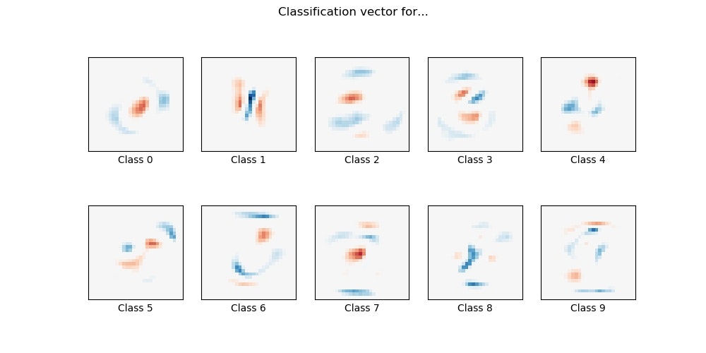
Test accuracyは0.84以上になっています。
L1正則化の下でWeightのスパース度(要素が0を取る率)が85.20%です。
>python scikit-learn-mnist.py
Using TensorFlow backend.
None
50000 train samples
10000 test samples
Sparsity with L1 penalty: 85.20%
Test score with L1 penalty: 0.8467
そして、以下のようにWeightの二次元画像が得られます。
coef = clf.coef_.copy()
plt.figure(figsize=(10, 5))
scale = np.abs(coef).max()
for i in range(10):
    l1_plot = plt.subplot(2, 5, i + 1)
    l1_plot.imshow(coef[i].reshape(28, 28), interpolation='nearest',
                   cmap=plt.cm.RdBu, vmin=-scale, vmax=scale)
    l1_plot.set_xticks(())
    l1_plot.set_yticks(())
    l1_plot.set_xlabel('Class %i' % i)
plt.suptitle('Classification vector for...')

run_time = time.time() - t0
print('Example run in %.3f s' % run_time)
plt.savefig('RFC/mnist_LR/logisticR_classification-vector'+str(train_samples)+'.jpg')
plt.show()
Example run in 20.018 s
None
Iteration 1, loss = 0.31528585
Iteration 2, loss = 0.23158923
Iteration 3, loss = 0.24815845
Iteration 4, loss = 0.21447691
Iteration 5, loss = 0.17414975
Iteration 6, loss = 0.19533443
Iteration 7, loss = 0.15429476
Iteration 8, loss = 0.14699409
Iteration 9, loss = 0.17666587
Iteration 10, loss = 0.14505811
Iteration 11, loss = 0.13630764
Iteration 12, loss = 0.11739588
Iteration 13, loss = 0.10552695
Iteration 14, loss = 0.08939208
Iteration 15, loss = 0.09680374
Iteration 16, loss = 0.09250149
Iteration 17, loss = 0.09477240
Training loss did not improve more than tol=0.000100 for two consecutive epochs. Stopping.
一方、いわゆるMLPでクラス分類を実施すると以下のようになります。
from sklearn.neural_network import MLPClassifier
print(__doc__)

# mlp = MLPClassifier(hidden_layer_sizes=(100, 100), max_iter=400, alpha=1e-4,
#                     solver='sgd', verbose=10, tol=1e-4, random_state=1)
mlp = MLPClassifier(hidden_layer_sizes=(50,), max_iter=20, alpha=1e-6,
                    solver='sgd', verbose=10, tol=1e-4, random_state=1,
                    learning_rate_init=.1)

mlp.fit(X_train, y_train)
print("Training set score: %f" % mlp.score(X_train, y_train))
print("Test set score: %f" % mlp.score(X_test, y_test))
fig, axes = plt.subplots(4, 4)
# use global min / max to ensure all weights are shown on the same scale
vmin, vmax = mlp.coefs_[0].min(), mlp.coefs_[0].max()
for coef, ax in zip(mlp.coefs_[0].T, axes.ravel()):
    ax.matshow(coef.reshape(28, 28), cmap=plt.cm.gray, vmin=.5 * vmin,
               vmax=.5 * vmax)
    ax.set_xticks(())
    ax.set_yticks(())
plt.savefig('RFC/mnist_LR/mnist_intermidiate-layer'+str(train_samples)+'.jpg')
plt.show()
中間層のWeightは以下のとおりになります。
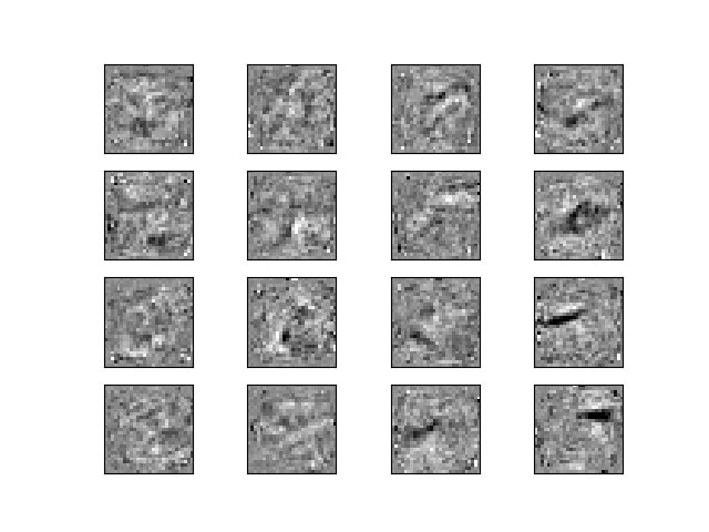
そして、精度は非常によく、95.8%が得られました。
Training set score: 0.984660
Test set score: 0.958200
KerasのMLPと上記のScikit-learnのMLPの比較
'''Trains a simple deep NN on the MNIST dataset.
Gets to 98.40% test accuracy after 20 epochs
(there is *a lot* of margin for parameter tuning).
2 seconds per epoch on a K520 GPU.
'''
from __future__ import print_function
import keras
from keras.datasets import mnist
from keras.models import Sequential
from keras.layers import Dense, Dropout
from keras.optimizers import RMSprop

batch_size = 128
num_classes = 10
epochs = 20
# the data, split between train and test sets
(x_train, y_train), (x_test, y_test) = mnist.load_data()
x_train = x_train.reshape(60000, 784)
x_test = x_test.reshape(10000, 784)
x_train = x_train.astype('float32')
x_test = x_test.astype('float32')
x_train /= 255
x_test /= 255
# convert class vectors to binary class matrices
y_train = keras.utils.to_categorical(y_train, num_classes)
y_test = keras.utils.to_categorical(y_test, num_classes)
モデルなどは以下のように出力されます。
>python mlp_scikit-learn+keras.py
Using TensorFlow backend.
60000 train samples
10000 test samples
_________________________________________________________________
Layer (type)                 Output Shape              Param #
=================================================================
dense_1 (Dense)              (None, 512)               401920
_________________________________________________________________
dropout_1 (Dropout)          (None, 512)               0
_________________________________________________________________
dense_2 (Dense)              (None, 512)               262656
_________________________________________________________________
dropout_2 (Dropout)          (None, 512)               0
_________________________________________________________________
dense_3 (Dense)              (None, 10)                5130
=================================================================
Total params: 669,706
Trainable params: 669,706
Non-trainable params: 0
_________________________________________________________________
Train on 60000 samples, validate on 10000 samples
model = Sequential()
model.add(Dense(512, activation='relu', input_shape=(784,)))
model.add(Dropout(0.2))
model.add(Dense(512, activation='relu'))
model.add(Dropout(0.2))
model.add(Dense(num_classes, activation='softmax'))

model.summary()

model.compile(loss='categorical_crossentropy',
              optimizer=RMSprop(),
              metrics=['accuracy'])
history = model.fit(x_train, y_train,
                    batch_size=batch_size,
                    epochs=epochs,
                    verbose=1,
                    validation_data=(x_test, y_test))
score = model.evaluate(x_test, y_test, verbose=0)
print('Test loss:', score[0])
print('Test accuracy:', score[1])
結果は、以下のように得られました。モデルは小さいですがとてもいいです。
Epoch 20/20
60000/60000 [==============================] - 2s 39us/step - loss: 0.0187 - acc: 0.9954 - val_loss: 0.1105 - val_acc: 0.9825
Test loss: 0.110451702557
Test accuracy: 0.9825
そして、同時実行したsklearnのMLPでは、以下の結果でした。
Training set score: 0.951433
Test set score: 0.937300
また、hidden_layer_sizes=(100, 100)では以下のとおりでした。
Iteration 32, loss = 0.00089717
Training loss did not improve more than tol=0.000100 for two consecutive epochs. Stopping.
Training set score: 1.000000
Test set score: 0.972800
import matplotlib.pyplot as plt
# from sklearn.datasets import fetch_openml
from sklearn.neural_network import MLPClassifier

print(__doc__)

# mlp = MLPClassifier(hidden_layer_sizes=(100, 100), max_iter=400, alpha=1e-4,
#                     solver='sgd', verbose=10, tol=1e-4, random_state=1)
mlp = MLPClassifier(hidden_layer_sizes=(50,), max_iter=10, alpha=1e-4,
                    solver='sgd', verbose=10, tol=1e-4, random_state=1,
                    learning_rate_init=.1)

mlp.fit(x_train, y_train)
print("Training set score: %f" % mlp.score(x_train, y_train))
print("Test set score: %f" % mlp.score(x_test, y_test))

fig, axes = plt.subplots(4, 4)
# use global min / max to ensure all weights are shown on the same scale
vmin, vmax = mlp.coefs_[0].min(), mlp.coefs_[0].max()
for coef, ax in zip(mlp.coefs_[0].T, axes.ravel()):
    ax.matshow(coef.reshape(28, 28), cmap=plt.cm.gray, vmin=.5 * vmin,
               vmax=.5 * vmax)
    ax.set_xticks(())
    ax.set_yticks(())
    plt.show()
・VGG16like(conv2dモデル)によるmnistの識別
最後にDeepLearningの代表格のVGG16で識別してみようと思います。
ただし、今回は入力が(28,28,1)と小さいので、block2までの小さなモデルで実施します。コードはおまけに記載しました。
結果は、Accuracy 99.56%で19s/epochを20epochの結果です。
Epoch 20/20
60000/60000 [==============================] - 19s 323us/step - loss: 0.0216 - acc: 0.9929 - val_loss: 0.0164 - val_acc: 0.9956
Test loss: 0.0164049295267
Test accuracy: 0.9956
モデルは以下のとおりです。
_________________________________________________________________
Layer (type)                 Output Shape              Param #
=================================================================
input_1 (InputLayer)         (None, 28, 28, 1)         0
_________________________________________________________________
conv1_1 (Conv2D)             (None, 28, 28, 64)        640
_________________________________________________________________
conv1_2 (Conv2D)             (None, 28, 28, 64)        36928
_________________________________________________________________
batch_normalization_1 (Batch (None, 28, 28, 64)        256
_________________________________________________________________
max_pooling2d_1 (MaxPooling2 (None, 14, 14, 64)        0
_________________________________________________________________
dropout_1 (Dropout)          (None, 14, 14, 64)        0
_________________________________________________________________
conv2_1 (Conv2D)             (None, 14, 14, 128)       73856
_________________________________________________________________
conv2_2 (Conv2D)             (None, 14, 14, 128)       147584
_________________________________________________________________
batch_normalization_2 (Batch (None, 14, 14, 128)       512
_________________________________________________________________
max_pooling2d_2 (MaxPooling2 (None, 7, 7, 128)         0
_________________________________________________________________
dropout_2 (Dropout)          (None, 7, 7, 128)         0
_________________________________________________________________
flatten_1 (Flatten)          (None, 6272)              0
_________________________________________________________________
dense_1 (Dense)              (None, 728)               4566744
_________________________________________________________________
activation_1 (Activation)    (None, 728)               0
_________________________________________________________________
dropout_3 (Dropout)          (None, 728)               0
_________________________________________________________________
dense_2 (Dense)              (None, 10)                7290
_________________________________________________________________
activation_2 (Activation)    (None, 10)                0
=================================================================
Total params: 4,833,810
Trainable params: 4,833,426
Non-trainable params: 384
_________________________________________________________________
Train on 60000 samples, validate on 10000 samples
まとめ
・機械学習の代表格のPCA+SVCとLogisticRegressionでMNISTデータのクラス分類を実施した
・Scikit-learnのMLPとKerasのMLPでMNISTデータのクラス分類を実施した
・VGG16ライクなモデルでDeepLearningでMNISTデータのクラス分類を実施した
・全体を並べて眺めると、機械学習とDeepLearningの精度の差がよくわかる
・学習時間はデータ数が多いとPCA+SVCが長時間計算が必要だが、それ以外はほとんど時間はかからない
・機械学習の小回りの良さとDeepLearningの精度の良さを利用したアプリへの適用が考えられる
おまけ
from __future__ import print_function
import keras
from keras.datasets import mnist
from keras.models import Sequential
from keras.layers import Dense, Dropout
from keras.optimizers import RMSprop

from keras.layers import BatchNormalization
from keras.layers import Activation, Flatten
from keras.layers import Conv2D, MaxPooling2D
from keras.layers import Input
from keras.models import Model
import h5py

batch_size = 128
num_classes = 10
epochs = 20

# the data, split between train and test sets
(x_train, y_train), (x_test, y_test) = mnist.load_data()

x_train = x_train.reshape(60000, 784)
x_test = x_test.reshape(10000, 784)
x_train = x_train.astype('float32')
x_test = x_test.astype('float32')
x_train /= 255
x_test /= 255
print(x_train.shape[0], 'train samples')
print(x_test.shape[0], 'test samples')

# convert class vectors to binary class matrices
y_train = keras.utils.to_categorical(y_train, num_classes)
y_test = keras.utils.to_categorical(y_test, num_classes)

def model_family_cnn(input_shape, num_classes=10):
    input_layer = Input(shape=input_shape)
    # Block 1
    conv1_1 = Conv2D(64, (3, 3),name='conv1_1', activation='relu', padding='same')(input_layer)
    conv1_2 = Conv2D(64, (3, 3),name='conv1_2', activation='relu', padding='same')(conv1_1)
    bn1 = BatchNormalization(axis=3)(conv1_2)
    pool1 = MaxPooling2D(pool_size=(2, 2))(bn1)
    drop1 = Dropout(0.5)(pool1)

    # Block 2
    conv2_1 = Conv2D(128, (3, 3),name='conv2_1', activation='relu', padding='same')(drop1)
    conv2_2 = Conv2D(128, (3, 3),name='conv2_2', activation='relu', padding='same')(conv2_1)
    bn2 = BatchNormalization(axis=3)(conv2_2)
    pool2 = MaxPooling2D(pool_size=(2, 2))(bn2)
    drop2 = Dropout(0.5)(pool2)

    x = Flatten()(drop2)
    x = Dense(728)(x)
    x = Activation('relu')(x)
    x = Dropout(0.5)(x)
    x = Dense(num_classes)(x)
    x = Activation('softmax')(x)
    model = Model(inputs=input_layer, outputs=x)
    return model

img_rows,img_cols=28, 28   #300, 300
input_shape = (img_rows,img_cols,1)   #224, 224, 3)

model = model_family_cnn(input_shape, num_classes = 10)
# optimizer adam
opt = keras.optimizers.Adam(lr=base_lr)

# load the weights from the last epoch
# model.load_weights('weights.hdf5', by_name=True)
print('Model loaded.')

# Let's train the model using RMSprop
model.compile(loss='categorical_crossentropy',
              optimizer=opt,
              metrics=['accuracy'])
model.summary()

x_train=x_train.reshape(60000,28,28,1)
x_test=x_test.reshape(10000,28,28,1)
model.fit(x_train, y_train,
          batch_size=batch_size,
          epochs=epochs,
          validation_data=(x_test, y_test),
          shuffle=True)
# save weights every epoch
model.save_weights('params_epoch_{0:03d}.hdf5'.format(epochs), True)

score = model.evaluate(x_test, y_test, verbose=0)
print('Test loss:', score[0])
print('Test accuracy:', score[1])