機械学習で、人の顔識別はちょっといい感じでできている。
【参考】
・①Faces recognition example using eigenfaces and SVMs
・②sklearn.neural_network.MLPClassifier
・③Visualization of MLP weights on MNIST
ちょっと前にもランダムフォレストやSVCで識別やったので、それらの発展形のようです。
また、さらに参考②でMLPが提供されており、さらに参考③ではそれを使って中間層のWeightの可視化を実施している。
やったこと
書いてみたら、長くなったので最初の項で切りました。
※続きは書いていきます。
・lfw_people.dataの識別とデータについて
・PCA+SVCによるmnistデータの識別
・MLPによるmnistの識別(・scikit-learn&keras)
・VGG16like(conv2dモデル)によるmnistの識別
・lfw_people.dataの識別とデータについて
scikit-learnで提供しているデータは、参考でまとめられている。
【参考】
・sklearn.datasets: Datasets
・fetch_lfw_people@5.3. Real world datasets@5. Dataset loading utilities
とりあえず、この中からリンクされている参考①についてみてみる。
これは以下のコードのとおり、PCA分析してその変換を実施したデータに対してSVCするという手法を取っている。
結果は参考と同じだけど、以下のように出力される。
※コードはまとめに置いておく
簡単にコードの説明すると、データを読み込んだあと、
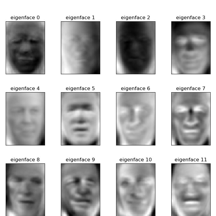
特徴成分n_components = 150(次元)としている。学習データをPCA(主成分分析)する。
そして、固有特徴成分を(h,w)にreshapeし、eigenfacesとする。ちなみにn_classes: 7である。データ読込が以下のとおり0.4で、画像の大きさはh: 50, w: 37であり、eigenfacesの個数は150個である。
そして、この特徴成分の寄与を以下の最後のコードのように出力してみると、最初の10個は以下のとおりであり、結構高次成分まで分布しているのが分かる。
pca.explained_variance_ratio_
[ 0.19334701  0.1512074   0.07087101  0.05948007  0.05157479  0.02887118
  0.02516412  0.02175809  0.02019792  0.01902673...]
lfw_people = fetch_lfw_people(min_faces_per_person=70, resize=0.4)
...
n_components = 150
print("Extracting the top %d eigenfaces from %d faces"
      % (n_components, X_train.shape[0]))
t0 = time()
pca = PCA(n_components=n_components, svd_solver='randomized',
          whiten=True).fit(X_train)
print("done in %0.3fs" % (time() - t0))
eigenfaces = pca.components_.reshape((n_components, h, w))
print("pca.explained_variance_ratio_{}".format(pca.explained_variance_ratio_))
そして、以下のように軸変換を実行し、SVCでClassificationします。
※ここではパラメーターC,gammaについてグリッドサーチしています。
print("Projecting the input data on the eigenfaces orthonormal basis")
X_train_pca = pca.transform(X_train)
X_test_pca = pca.transform(X_test)
param_grid = {'C': [1e3, 5e3, 1e4, 5e4, 1e5],
              'gamma': [0.0001, 0.0005, 0.001, 0.005, 0.01, 0.1], }
clf = GridSearchCV(SVC(kernel='rbf', class_weight='balanced'),
                   param_grid, cv=5)
clf = clf.fit(X_train_pca, y_train)
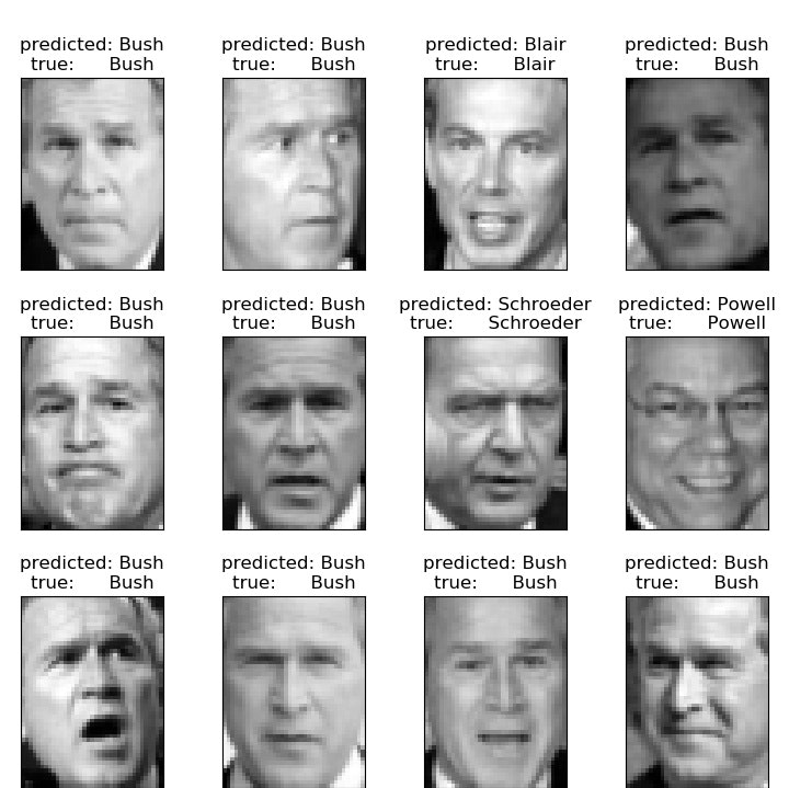
こうして以下のように写真の名前を予測することができます。
print("Predicting people's names on the test set")
y_pred = clf.predict(X_test_pca)

print(classification_report(y_test, y_pred, target_names=target_names))
print(confusion_matrix(y_test, y_pred, labels=range(n_classes)))
まとめ
・PCA+SVCによる顔の識別を解説しました
次回はmnistデータへの応用から入ります
おまけ
理解のためのコードを残しています。
from __future__ import print_function

from time import time
import logging
import matplotlib.pyplot as plt

from sklearn.model_selection import train_test_split
from sklearn.model_selection import GridSearchCV
from sklearn.datasets import fetch_lfw_people
from sklearn.metrics import classification_report
from sklearn.metrics import confusion_matrix
from sklearn.decomposition import PCA
from sklearn.svm import SVC

print(__doc__)

# Display progress logs on stdout
logging.basicConfig(level=logging.INFO, format='%(asctime)s %(message)s')

# #############################################################################
# Download the data, if not already on disk and load it as numpy arrays

lfw_people = fetch_lfw_people(min_faces_per_person=70, resize=0.4)

# introspect the images arrays to find the shapes (for plotting)
n_samples, h, w = lfw_people.images.shape

# for machine learning we use the 2 data directly (as relative pixel
# positions info is ignored by this model)
X = lfw_people.data
n_features = X.shape[1]

# the label to predict is the id of the person
y = lfw_people.target
target_names = lfw_people.target_names
n_classes = target_names.shape[0]

print("Total dataset size:")
print("n_samples: %d" % n_samples)
print("n_features: %d" % n_features)
print("n_classes: %d" % n_classes)
# print("h: {}, w: {}".format(h,w))

# #############################################################################
# Split into a training set and a test set using a stratified k fold

# split into a training and testing set
X_train, X_test, y_train, y_test = train_test_split(
    X, y, test_size=0.25, random_state=42)

# #############################################################################
# Compute a PCA (eigenfaces) on the face dataset (treated as unlabeled
# dataset): unsupervised feature extraction / dimensionality reduction
n_components = 150

print("Extracting the top %d eigenfaces from %d faces"
      % (n_components, X_train.shape[0]))
t0 = time()
pca = PCA(n_components=n_components, svd_solver='randomized',
          whiten=True).fit(X_train)
print("done in %0.3fs" % (time() - t0))

eigenfaces = pca.components_.reshape((n_components, h, w))
print("eigenfaces={}".format(len(eigenfaces)))
print("eigenfaces={}".format(eigenfaces))
"""
for i in range(5):
    plt.imshow(eigenfaces[i].reshape((h, w)), cmap=plt.cm.gray)
    plt.pause(0.5)
    plt.close()
"""
print("Projecting the input data on the eigenfaces orthonormal basis")
t0 = time()
X_train_pca = pca.transform(X_train)
X_test_pca = pca.transform(X_test)
"""
for i in range(3):
    print("X_train_pca[i]={}".format(X_train_pca[i]))
    print("y_train[i]={}".format(y_train[i]))
"""
print("done in %0.3fs" % (time() - t0))
print("pca.explained_variance_ratio_{}".format(pca.explained_variance_ratio_))

# #############################################################################
# Train a SVM classification model

print("Fitting the classifier to the training set")
t0 = time()
param_grid = {'C': [1e3, 5e3, 1e4, 5e4, 1e5],
              'gamma': [0.0001, 0.0005, 0.001, 0.005, 0.01, 0.1], }
clf = GridSearchCV(SVC(kernel='rbf', class_weight='balanced'),
                   param_grid, cv=5)
clf = clf.fit(X_train_pca, y_train)
print("done in %0.3fs" % (time() - t0))
print("Best estimator found by grid search:")
print(clf.best_estimator_)

# #############################################################################
# Quantitative evaluation of the model quality on the test set

print("Predicting people's names on the test set")
t0 = time()
y_pred = clf.predict(X_test_pca)
print("done in %0.3fs" % (time() - t0))

print(classification_report(y_test, y_pred, target_names=target_names))
print(confusion_matrix(y_test, y_pred, labels=range(n_classes)))


# #############################################################################
# Qualitative evaluation of the predictions using matplotlib

def plot_gallery(images, titles, h, w, n_row=3, n_col=4):
    """Helper function to plot a gallery of portraits"""
    plt.figure(figsize=(1.8 * n_col, 2.4 * n_row))
    plt.subplots_adjust(bottom=0, left=.01, right=.99, top=.90, hspace=.35)
    for i in range(n_row * n_col):
        plt.subplot(n_row, n_col, i + 1)
        plt.imshow(images[i].reshape((h, w)), cmap=plt.cm.gray)
        plt.title(titles[i], size=12)
        plt.xticks(())
        plt.yticks(())

# plot the result of the prediction on a portion of the test set
def title(y_pred, y_test, target_names, i):
    pred_name = target_names[y_pred[i]].rsplit(' ', 1)[-1]
    true_name = target_names[y_test[i]].rsplit(' ', 1)[-1]
    return 'predicted: %s\ntrue:      %s' % (pred_name, true_name)

prediction_titles = [title(y_pred, y_test, target_names, i)
                     for i in range(y_pred.shape[0])]

plot_gallery(X_test, prediction_titles, h, w)
plt.savefig('RFC/mnist_PCAKmeans/PCASVC_peaple_Xtest.jpg')
plt.pause(1)
plt.close()
# plot the gallery of the most significative eigenfaces

eigenface_titles = ["eigenface %d" % i for i in range(eigenfaces.shape[0])]
plot_gallery(eigenfaces, eigenface_titles, h, w)
plt.savefig('RFC/mnist_PCAKmeans/PCASVC_peaple_eigenface.jpg')
plt.pause(1)
plt.close()