昨夜で、【データサイエンティスト入門】科学計算、データ加工、グラフ描画ライブラリの使い方の基礎までまとめました。今夜からいよいよそれらを使って本題に入っていきます。今夜は記述統計と単回帰分析をまとめます。本書に乗った解説を補足することとします。
【注意】
「東京大学のデータサイエンティスト育成講座」を読んで、ちょっと疑問を持ったところや有用だと感じた部分をまとめて行こうと思う。
したがって、あらすじはまんまになると思うが内容は本書とは関係ないと思って読んでいただきたい。
Chapter 3 記述統計と単回帰分析
Chapter 3-1 統計解析の種類
3-1-1 記述統計と推論統計
統計解析の手法は、記述統計と推論統計に分かれる。
3-1-1-1 記述統計
「集めたデータの特徴をつかんだり分かり易く整理したり見やすくしたりする方法。平均、標準偏差などを計算してデータの特徴を計算したり、データを分類したり、図やグラフを用いて表現したりするのが、記述統計です。」
3-1-1-2 推論統計
「部分的なデータしかないものから、確率分布に基いたモデルを用いて精密な解析をし、全体を推論して統計を求めるのが推論統計の考え方です。」
「過去のデータから未来予測するときにも使われます。この章では、推論統計の基礎である単回帰分析について説明します。より複雑な推論統計については、次の4章で扱います。」
3-1-2 ライブラリのインポート
import numpy as np
import scipy as sp
import pandas as pd
from pandas import Series, DataFrame

import matplotlib as mpl
import seaborn as sns
import matplotlib.pyplot as plt
sns.set()

from sklearn import linear_model
$ sudo pip3 install scikit-learn
以下のとおり、Rasipi4でも使えそうです。
 $ python3
Python 3.7.3 (default, Jul 25 2020, 13:03:44)
[GCC 8.3.0] on linux
Type "help", "copyright", "credits" or "license" for more information.
>>> from sklearn import linear_model
>>>
一応、python3-sklearn-docが見つかりませんでしたがDebian/Ubuntuの以下でもインストール出来たようです。
$ sudo apt-get install python3-sklearn python3-sklearn-lib
※検証は以下単回帰分析のとき問題でるかを見ていきます
Chapter 3-2 データの読込と対話
...省略
3-2-1-5
以下のサイトから、以下のプログラムでデータstudent.zipを取得します。
https://archive.ics.uci.edu/ml/machine-learning-databases/00356/student.zip
import requests, zipfile
from io import StringIO
import io

url = 'https://archive.ics.uci.edu/ml/machine-learning-databases/00356/student.zip'
r = requests.get(url, stream = True)
z = zipfile.ZipFile(io.BytesIO(r.content))
z.extractall()
以下の4つのファイルが展開されました。
student.txt
student-mat.csv
student-merge.R
student-pcr.csv
3-2-2 データ読み込みと確認
上記importにつなげて、以下を実行
student_data_math = pd.read_csv('./chap3/student-mat.csv')
print(student_data_math.head())
データが ;区切りを確認できる。
school;sex;age;address;famsize;Pstatus;Medu;Fedu;Mjob;Fjob;reason;guardian;traveltime;studytime;failures;schoolsup;famsup;paid;activities;nursery;higher;internet;romantic;famrel;freetime;goout;Dalc;Walc;health;absences;G1;G2;G3
0  GP;"F";18;"U";"GT3";"A";4;4;"at_home";"teacher...
1  GP;"F";17;"U";"GT3";"T";1;1;"at_home";"other";...
2  GP;"F";15;"U";"LE3";"T";1;1;"at_home";"other";...
3  GP;"F";15;"U";"GT3";"T";4;2;"health";"services...
4  GP;"F";16;"U";"GT3";"T";3;3;"other";"other";"h...
読込を ;に変更して再読み込み。
student_data_math = pd.read_csv('./chap3/student-mat.csv', sep =';')
print(student_data_math.head())
綺麗に見えた。
  school sex  age address famsize Pstatus  Medu  Fedu  ... goout Dalc Walc health  absences  G1  G2  G3
0     GP   F   18       U     GT3       A     4     4  ...     4    1    1      3         6   5   6   6
1     GP   F   17       U     GT3       T     1     1  ...     3    1    1      3         4   5   5   6
2     GP   F   15       U     LE3       T     1     1  ...     2    2    3      3        10   7   8  10
3     GP   F   15       U     GT3       T     4     2  ...     2    1    1      5         2  15  14  15
4     GP   F   16       U     GT3       T     3     3  ...     2    1    2      5         4   6  10  10

[5 rows x 33 columns]
3-2-3 データの性質を確認する
print(student_data_math.info())
<class 'pandas.core.frame.DataFrame'>
RangeIndex: 395 entries, 0 to 394
Data columns (total 33 columns):
 #   Column      Non-Null Count  Dtype
---  ------      --------------  -----
 0   school      395 non-null    object
 1   sex         395 non-null    object
 2   age         395 non-null    int64
 3   address     395 non-null    object
 4   famsize     395 non-null    object
 5   Pstatus     395 non-null    object
 6   Medu        395 non-null    int64
 7   Fedu        395 non-null    int64
 8   Mjob        395 non-null    object
 9   Fjob        395 non-null    object
 10  reason      395 non-null    object
 11  guardian    395 non-null    object
 12  traveltime  395 non-null    int64
 13  studytime   395 non-null    int64
 14  failures    395 non-null    int64
 15  schoolsup   395 non-null    object
 16  famsup      395 non-null    object
 17  paid        395 non-null    object
 18  activities  395 non-null    object
 19  nursery     395 non-null    object
 20  higher      395 non-null    object
 21  internet    395 non-null    object
 22  romantic    395 non-null    object
 23  famrel      395 non-null    int64
 24  freetime    395 non-null    int64
 25  goout       395 non-null    int64
 26  Dalc        395 non-null    int64
 27  Walc        395 non-null    int64
 28  health      395 non-null    int64
 29  absences    395 non-null    int64
 30  G1          395 non-null    int64
 31  G2          395 non-null    int64
 32  G3          395 non-null    int64
dtypes: int64(16), object(17)
memory usage: 102.0+ KB
cat student.txtして、中身を見るとこのデータは以下のような内容だそうです。
※本書では翻訳されています
$ cat student.txt
# Attributes for both student-mat.csv (Math course) and student-por.csv (Portuguese language course) datasets:
1 school - student's school (binary: "GP" - Gabriel Pereira or "MS" - Mousinho da Silveira)
2 sex - student's sex (binary: "F" - female or "M" - male)
3 age - student's age (numeric: from 15 to 22)
4 address - student's home address type (binary: "U" - urban or "R" - rural)
5 famsize - family size (binary: "LE3" - less or equal to 3 or "GT3" - greater than 3)
6 Pstatus - parent's cohabitation status (binary: "T" - living together or "A" - apart)
7 Medu - mother's education (numeric: 0 - none,  1 - primary education (4th grade), 2 – 5th to 9th grade, 3 – secondary education or 4 – higher education)
8 Fedu - father's education (numeric: 0 - none,  1 - primary education (4th grade), 2 – 5th to 9th grade, 3 – secondary education or 4 – higher education)
9 Mjob - mother's job (nominal: "teacher", "health" care related, civil "services" (e.g. administrative or police), "at_home" or "other")
10 Fjob - father's job (nominal: "teacher", "health" care related, civil "services" (e.g. administrative or police), "at_home" or "other")
11 reason - reason to choose this school (nominal: close to "home", school "reputation", "course" preference or "other")
12 guardian - student's guardian (nominal: "mother", "father" or "other")
13 traveltime - home to school travel time (numeric: 1 - <15 min., 2 - 15 to 30 min., 3 - 30 min. to 1 hour, or 4 - >1 hour)
14 studytime - weekly study time (numeric: 1 - <2 hours, 2 - 2 to 5 hours, 3 - 5 to 10 hours, or 4 - >10 hours)
15 failures - number of past class failures (numeric: n if 1<=n<3, else 4)
16 schoolsup - extra educational support (binary: yes or no)
17 famsup - family educational support (binary: yes or no)
18 paid - extra paid classes within the course subject (Math or Portuguese) (binary: yes or no)
19 activities - extra-curricular activities (binary: yes or no)
20 nursery - attended nursery school (binary: yes or no)
21 higher - wants to take higher education (binary: yes or no)
22 internet - Internet access at home (binary: yes or no)
23 romantic - with a romantic relationship (binary: yes or no)
24 famrel - quality of family relationships (numeric: from 1 - very bad to 5 - excellent)
25 freetime - free time after school (numeric: from 1 - very low to 5 - very high)
26 goout - going out with friends (numeric: from 1 - very low to 5 - very high)
27 Dalc - workday alcohol consumption (numeric: from 1 - very low to 5 - very high)
28 Walc - weekend alcohol consumption (numeric: from 1 - very low to 5 - very high)
29 health - current health status (numeric: from 1 - very bad to 5 - very good)
30 absences - number of school absences (numeric: from 0 to 93)

# these grades are related with the course subject, Math or Portuguese:
31 G1 - first period grade (numeric: from 0 to 20)
31 G2 - second period grade (numeric: from 0 to 20)
32 G3 - final grade (numeric: from 0 to 20, output target)

Additional note: there are several (382) students that belong to both datasets .
These students can be identified by searching for identical attributes
that characterize each student, as shown in the annexed R file.
3-2-4 量的データと質的データ
・量的データ
四則演算を適用可能な連続値で表現されるデータであり、比率に意味がある。例;人数、金額など
・質的データ
四則演算を適用不可能な不連続のデータであり、状態を表現するために利用される。
例;順位、カテゴリなど
性別は質的データ
print(student_data_math['sex'].head())
0    F
1    F
2    F
3    F
4    F
Name: sex, dtype: object
欠席数は量的データ
print(student_data_math['absences'].head())
0     6
1     4
2    10
3     2
4     4
Name: absences, dtype: int64
3-2-4-2 軸別に平均値を求める
print(student_data_math.groupby('sex')['age'].mean())
sex
F    16.730769
M    16.657754
Name: age, dtype: float64
女性の方が勉強する。
print(student_data_math.groupby('sex')['studytime'].mean())
sex
F    2.278846
M    1.764706
Name: studytime, dtype: float64
記述統計
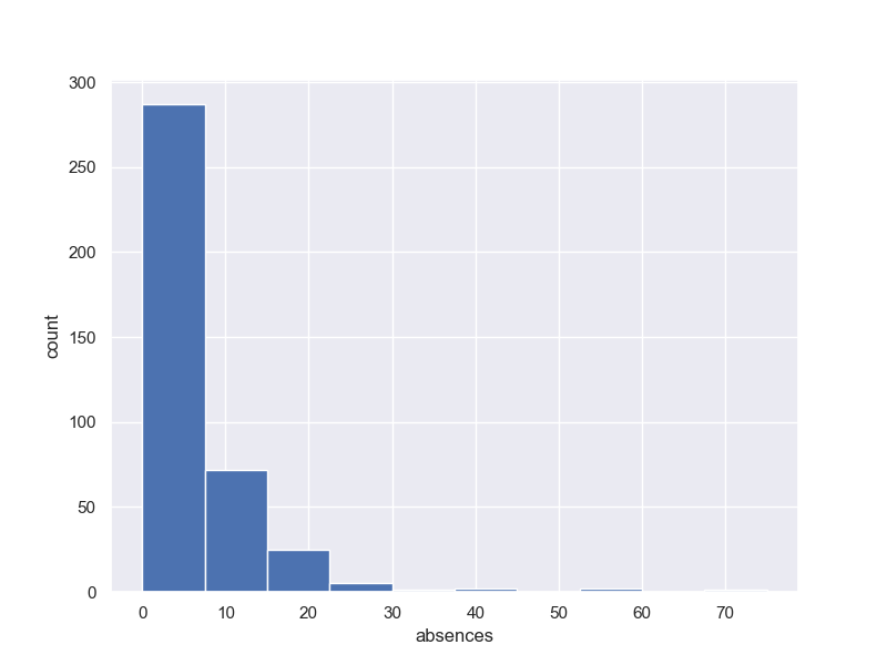
3-3-1 ヒストグラム
fig, (ax1) = plt.subplots(1, 1, figsize=(8,6))
y1 = student_data_math['absences']
ax1.hist(y1, bins = 10, range =(0.0,max(y1)))
ax1.set_ylabel('count')
ax1.set_xlabel('absences')
plt.grid(True)
plt.show()
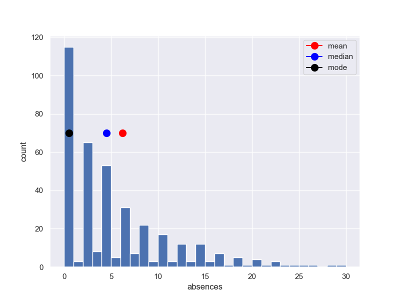
3-3-2 平均値、中央値、最頻値
print('平均値{}'.format(student_data_math['absences'].mean()))
print('中央値{}'.format(student_data_math['absences'].median()))
print('最頻値{}'.format(student_data_math['absences'].mode()))

平均値5.708860759493671
中央値4.0
最頻値0    0
dtype: int64
図で検証するために、上記を図を拡大して記入します。
※横軸0.5修正しています。
fig, (ax1) = plt.subplots(1, 1, figsize=(8,6))
y1 = student_data_math['absences']
ax1.hist(y1, bins = 30, range =(0.0,30))  #,max(y1)
x0 = student_data_math['absences'].mean()
ax1.plot(x0+0.5, 70,  'red', marker = 'o',markersize=10,label ='mean')
x0 = student_data_math['absences'].median()
ax1.plot(x0+0.5, 70, 'blue', marker = 'o',markersize=10,label ='median')
x0 = student_data_math['absences'].mode()
ax1.plot(x0+0.5, 70, 'black', marker = 'o',markersize=10,label ='mode')
ax1.legend()
ax1.set_ylabel('count')
ax1.set_xlabel('absences')
plt.grid(True)
plt.show()
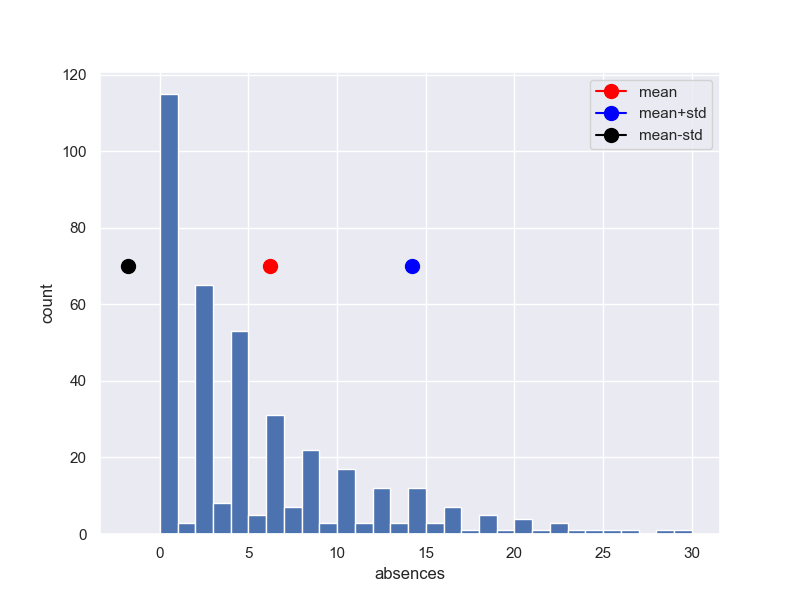
3-3-3 分散と標準偏差
定義式
分散$σ^2$
σ^2 = \frac{1}{n}\Sigma_{i=1}^{n}(x_i-\bar{x})^2
標準偏差$σ$
std(standered deviation)
σ = \sqrt{\frac{1}{n}\Sigma_{i=1}^{n}(x_i-\bar{x})^2}
print('分散{}'.format(student_data_math['absences'].var(ddof=0)))
print('標準偏差{}'.format(student_data_math['absences'].std(ddof = 0)))
print('標準偏差{}'.format(np.sqrt(student_data_math['absences'].var())))
分散63.887389841371565
標準偏差7.99295876640006
標準偏差8.00309568710818
平均±標準偏差をプロットする。
fig, (ax1) = plt.subplots(1, 1, figsize=(8,6))
y1 = student_data_math['absences']
ax1.hist(y1, bins = 30, range =(0.0,30))  #,max(y1)
x0 = student_data_math['absences'].mean()
ax1.plot(x0+0.5, 70,  'red', marker = 'o',markersize=10,label ='mean')
x1 = student_data_math['absences'].std(ddof=0)
ax1.plot(x0+x1+0.5, 70, 'blue', marker = 'o',markersize=10,label ='mean+std')
ax1.plot(x0-x1+0.5, 70, 'black', marker = 'o',markersize=10,label ='mean-std')
ax1.legend()
ax1.set_ylabel('count')
ax1.set_xlabel('absences')
plt.grid(True)
plt.show()
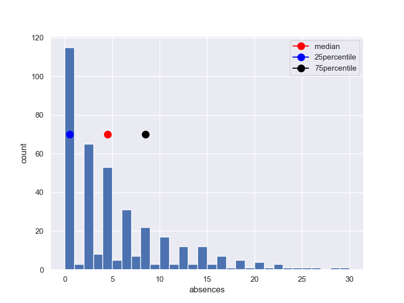
3-3-4 要約統計量とパーセンタイル値
パーセンタイル値は全体数を100とした時の順位
25番目を25パーセンタイル、第一四分位点
75番目を75パーセンタイル、第三四分位点
50パーセンタイル値、中央値
print('要約統計量', student_data_math['absences'].describe())
要約統計量 count    395.000000
mean       5.708861
std        8.003096
min        0.000000
25%        0.000000
50%        4.000000
75%        8.000000
max       75.000000
Name: absences, dtype: float64
四分位範囲を求める
25パーセンタイル;describe(4)
75パーセンタイル:describe(6)
差;describe(6)-describe(4)
print('75-25パーセンタイル', student_data_math['absences'].describe()[6]-student_data_math['absences'].describe()[4])
75-25パーセンタイル 8.0
fig, (ax1) = plt.subplots(1, 1, figsize=(8,6))
y1 = student_data_math['absences']
ax1.hist(y1, bins = 30, range =(0.0,30))  #,max(y1)
x0 = student_data_math['absences'].median()
ax1.plot(x0+0.5, 70,  'red', marker = 'o',markersize=10,label ='median')
x1 = student_data_math['absences'].describe()[4]
ax1.plot(x1+0.5, 70, 'blue', marker = 'o',markersize=10,label ='25percentile')
x1 = student_data_math['absences'].describe()[6]
ax1.plot(x1+0.5, 70, 'black', marker = 'o',markersize=10,label ='75percentile')
ax1.legend()
ax1.set_ylabel('count')
ax1.set_xlabel('absences')
plt.grid(True)
plt.show()
3-3-4-2 全列のdescribe()
print('全列要約統計量', student_data_math.describe())
全列要約統計量
              age        Medu        Fedu  traveltime  ...    absences          G1          G2          G3
count  395.000000  395.000000  395.000000  395.000000  ...  395.000000  395.000000  395.000000  395.000000
mean    16.696203    2.749367    2.521519    1.448101  ...    5.708861   10.908861   10.713924   10.415190
std      1.276043    1.094735    1.088201    0.697505  ...    8.003096    3.319195    3.761505    4.581443
min     15.000000    0.000000    0.000000    1.000000  ...    0.000000    3.000000    0.000000    0.000000
25%     16.000000    2.000000    2.000000    1.000000  ...    0.000000    8.000000    9.000000    8.000000
50%     17.000000    3.000000    2.000000    1.000000  ...    4.000000   11.000000   11.000000   11.000000
75%     18.000000    4.000000    3.000000    2.000000  ...    8.000000   13.000000   13.000000   14.000000
max     22.000000    4.000000    4.000000    4.000000  ...   75.000000   19.000000   19.000000   20.000000

[8 rows x 16 columns]
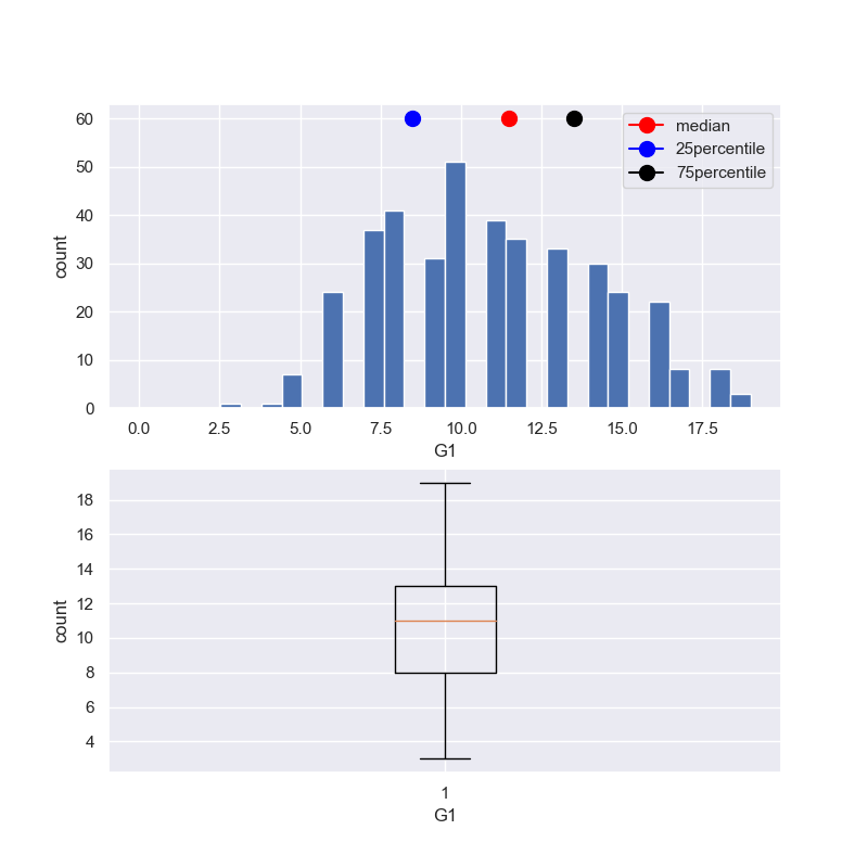
3-3-5 箱ひげ図
箱ひげ図は、(最小値,第1四分位点,中央値,第3四分位点,最大値)で以下のように箱とひげで表す手法。
fig, (ax1,ax2) = plt.subplots(2, 1, figsize=(8,2*4))
y1 = student_data_math['G1']
ax1.hist(y1, bins = 30, range =(0.0,max(y1)))  #,max(y1)
x0 = student_data_math['G1'].median()
ax1.plot(x0+0.5, 60,  'red', marker = 'o',markersize=10,label ='median')
x1 = student_data_math['G1'].describe()[4]
ax1.plot(x1+0.5, 60, 'blue', marker = 'o',markersize=10,label ='25percentile')
x1 = student_data_math['G1'].describe()[6]
ax1.plot(x1+0.5, 60, 'black', marker = 'o',markersize=10,label ='75percentile')
ax2.boxplot(y1)
ax2.set_xlabel('G1')
ax2.set_ylabel('count')
ax1.legend()
ax1.set_ylabel('count')
ax1.set_xlabel('G1')
plt.grid(True)
plt.show()
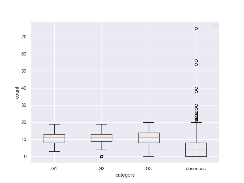
fig, (ax1) = plt.subplots(1, 1, figsize=(8,6))
y1 = [student_data_math['G1'],student_data_math['G2'],student_data_math['G3'],student_data_math['absences']]
ax1.boxplot(y1,labels=['G1', 'G2', 'G3', 'absences'])
ax1.set_xlabel('category')
ax1.set_ylabel('count')
ax1.legend()
ax1.set_ylabel('count')
ax1.set_xlabel('category')
plt.grid(True)
plt.show()
3-3-6 変動係数
変動係数CVとは、標準偏差σ/平均値$\bar{x}$
変動係数は、スケールに依存せず、散らばり具合が分かる。
print(student_data_math.std()/student_data_math.mean())
age           0.076427
Medu          0.398177
Fedu          0.431565
traveltime    0.481668
studytime     0.412313
failures      2.225319
famrel        0.227330
freetime      0.308725
goout         0.358098
Dalc          0.601441
Walc          0.562121
health        0.391147
absences      1.401873
G1            0.304266
G2            0.351086
G3            0.439881
dtype: float64
3-3-7 散布図と相関係数
fig, (ax1) = plt.subplots(1, 1, figsize=(8,6))
x = student_data_math['G1']
y = student_data_math['G3']
ax1.plot(x,y, 'o')
ax1.set_xlabel('G1-grade')
ax1.set_ylabel('G3-grade')
ax1.legend()
plt.grid(True)
plt.show()
G1-Gradeの高かった人は、G3-Gradeも高い。
ただし、G3-Gradeが0の人が数人出ている。これは、異常値だが、理由はいろいろちゅさして、除外するかどうか決めようという議論がされている。
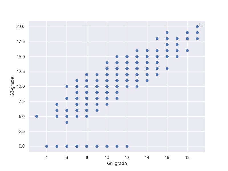
そこで、G3-Gradeが0の人の出席日数はどうなのということで、以下の相関図を描いて見る。
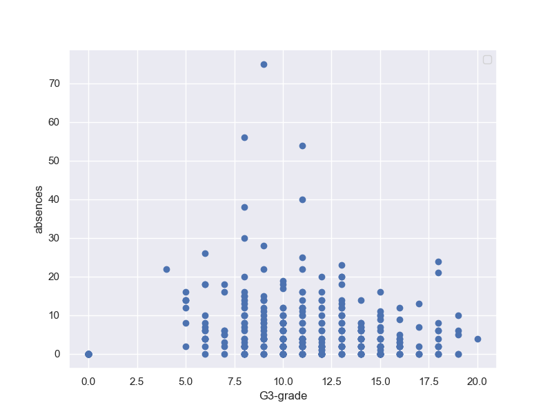
fig, (ax1) = plt.subplots(1, 1, figsize=(8,6))
x = student_data_math['G3']
y = student_data_math['absences']
ax1.plot(x,y, 'o')
ax1.set_xlabel('G3-grade')
ax1.set_ylabel('absences')
ax1.legend()
plt.grid(True)
plt.show()
結果は、G3-Gradeが0の人は欠席0という結果。なんかおかしい。実は、途中でやめてノーカウントなのではとか想像できる。
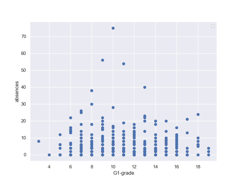
さらに、G1-Gradeと欠席数で相関取ると、以下の通り
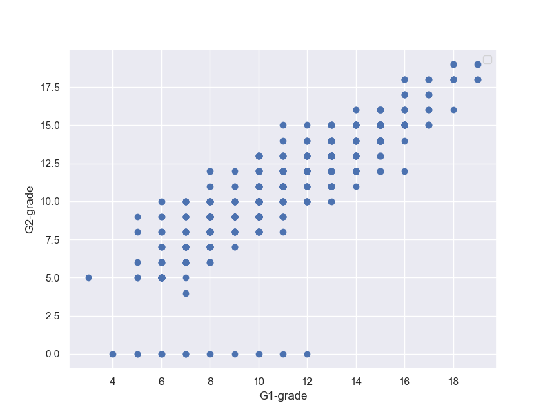
そもそも、G2-Gradeの時点で数名が0Gradeになっている。
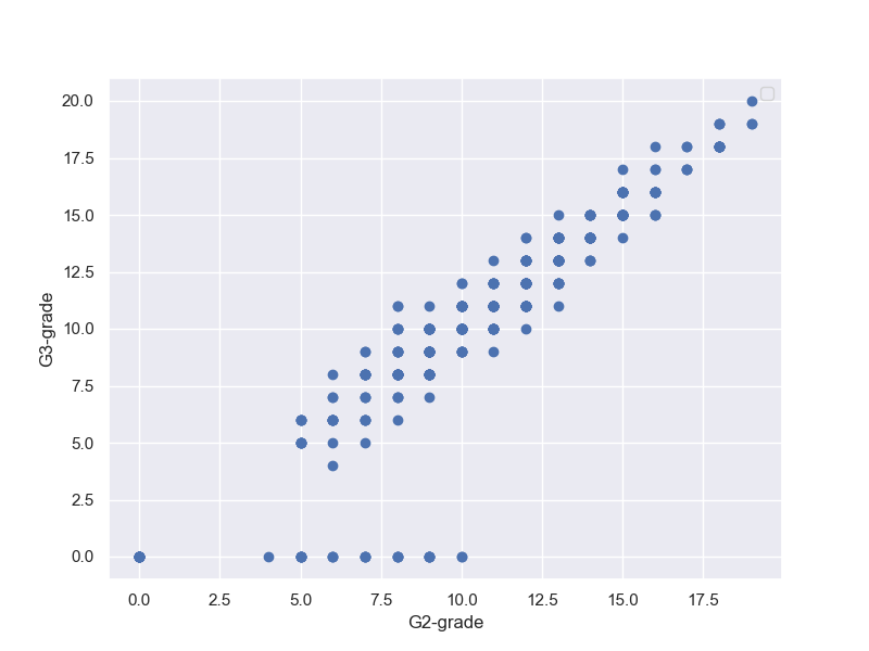
そして、G2-GradeとG3-Gradeの相関見ても、何人かは0Gradeに転落しており、そういう人も段々増えていることが分かる。そして、落伍者は点数の低めの人の中から出ているようだ。
だから、一つのグラフで結論を急ぐよりも、いろいろデータを分析することも大切だと言える。
3-3-7-1 共分散
定義式は、以下の通り
S_{xy}=\frac{1}{n}\Sigma_{i=1}^{n}(x_i-\bar{x})(y_i-\bar{y})
すなわち、対角項は上で定義した分散になります。
では、非対角項は何を意味するのでしょう。
参考によれば、$x$と$y$が本来線形な関係があるとすると、最小二乗法で導かれる直線の方程式は以下となる。
【参考】
線形回帰分析・最小二乗法とは 共分散・相関係数の意味
y=\frac{S_{xy}}{\sigma^2_{x}}x + \bar y−\frac{S_{xy}}{\sigma^2_x}\bar x \\
変形すると、\\
\frac{y-\bar y}{\sigma_y}=\frac{S_{xy}}{\sigma_x\sigma_y}\frac{x-\bar x}{\sigma_x}
すなわち、標準偏差と平均値で規格化した一次方程式の傾きは以下の式となります。
r_{xy}=\frac{S_{xy}}{\sigma_x\sigma_y}
すなわち、共分散を標準偏差で規格化した値になり、これがいわゆる相関係数$r_{xy}$の定義式です。
3-3-7-2 相関係数
ここでは、共分散と相関係数を求めます。
共分散は、非対角項、対角項はG1,G3の分散です。
print(np.cov(student_data_math['G1'],student_data_math['G3']))
[[11.01705327 12.18768232]
 [12.18768232 20.9896164 ]]
相関係数は、前が相関係数、第二項はp値です。
※p値については後ろの章で取り上げる予定
print(sp.stats.pearsonr(student_data_math['G1'],student_data_math['G3']))
(0.801467932017414, 9.001430312277865e-90)
相関行列は、以下で求められます。
print(np.corrcoef(student_data_math['G1'],student_data_math['G3']))
[[1.         0.80146793]
 [0.80146793 1.        ]]
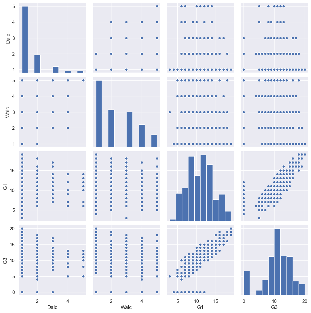
3-3-8 すべての変数のヒストグラムや散布図を描く
Dalc;平日のアルコール摂取量
Walc;週末のアルコール摂取量
とG1,G3の得点に相関はあるか、散布図を描いて見る。
結果;無さそう
g = sns.pairplot(student_data_math[['Dalc','Walc','G1','G3']])
g.savefig('seaborn_pairplot_g.png')
【参考】
Python, pandas, seabornでペアプロット図(散布図行列)を作成
WalcとG3得点の相関無し
print(np.corrcoef(student_data_math['Walc'],student_data_math['G3']))
[[ 1.         -0.05193932]
 [-0.05193932  1.        ]]
グループ毎のバラツキ無し
print(student_data_math.groupby('Walc')['G3'].mean())
Walc
1    10.735099
2    10.082353
3    10.725000
4     9.686275
5    10.142857
Name: G3, dtype: float64
練習問題3-1
              age        Medu        Fedu  traveltime  ...    absences          G1          G2          G3
count  649.000000  649.000000  649.000000  649.000000  ...  649.000000  649.000000  649.000000  649.000000
mean    16.744222    2.514638    2.306626    1.568567  ...    3.659476   11.399076   11.570108   11.906009
std      1.218138    1.134552    1.099931    0.748660  ...    4.640759    2.745265    2.913639    3.230656
min     15.000000    0.000000    0.000000    1.000000  ...    0.000000    0.000000    0.000000    0.000000
25%     16.000000    2.000000    1.000000    1.000000  ...    0.000000   10.000000   10.000000   10.000000
50%     17.000000    2.000000    2.000000    1.000000  ...    2.000000   11.000000   11.000000   12.000000
75%     18.000000    4.000000    3.000000    2.000000  ...    6.000000   13.000000   13.000000   14.000000
max     22.000000    4.000000    4.000000    4.000000  ...   32.000000   19.000000   19.000000   19.000000
練習問題3-2
df =student_data_math.merge(student_data_por,left_on=['school','sex','age','address','famsize','Pstatus','Medu','Fedu','Mjob','Fjob','reason','nursery','internet'], right_on=['school','sex','age','address','famsize','Pstatus','Medu','Fedu','Mjob','Fjob','reason','nursery','internet'], suffixes=('_math', '_por'))
print(df.head())
  school sex  age address famsize Pstatus  ...  Walc_por  health_por absences_por G1_por G2_por G3_por
0     GP   F   18       U     GT3       A  ...         1           3            4      0     11     11
1     GP   F   17       U     GT3       T  ...         1           3            2      9     11     11
2     GP   F   15       U     LE3       T  ...         3           3            6     12     13     12
3     GP   F   15       U     GT3       T  ...         1           5            0     14     14     14
4     GP   F   16       U     GT3       T  ...         2           5            0     11     13     13

[5 rows x 53 columns]
練習問題3-3
gm = sns.pairplot(df[['G1_math','G3_math','G1_por','G3_por']])
gm.savefig('seaborn_pairplot_gm.png')
mathどうし、porどうしの相関が高そう
mathよりporの方が分散は小さそう
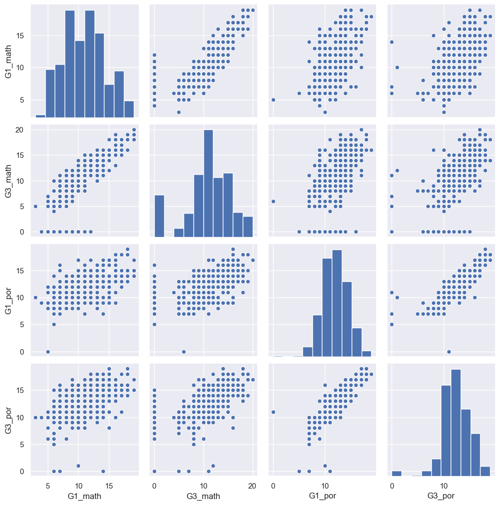
以下の結果からも裏付けられる。
print(np.corrcoef(df['G1_math'],df['G3_math']))
[[1.        0.8051287]
 [0.8051287 1.       ]]
print(np.corrcoef(df['G3_math'],df['G3_por']))
[[1.         0.48034936]
 [0.48034936 1.        ]]

print(np.cov(df['G1_math'],df['G3_math']))
[[11.2169202  12.63919693]
 [12.63919693 21.9702354 ]]
print(np.cov(df['G3_math'],df['G3_por']))
[[21.9702354   6.63169394]
 [ 6.63169394  8.67560567]]
Chapter 3-4 単回帰分析
「記述統計の次は、回帰分析の基礎を学びましょう。」
「回帰分析とは、数値を予測する分析です。...上の学生のデータについて、グラフ化しました。この散布図から、G1とG3には関係がありそうだというのは分かります。」
fig, (ax1) = plt.subplots(1, 1, figsize=(8,6))
ax1.plot(student_data_math['G1'],student_data_math['G3'],'o')
ax1.set_xlabel('G1_Grade')
ax1.set_ylabel('G3_Grade')
ax1.grid(True)
plt.show()

「回帰問題では、与えられたデータから関係式を仮定して、データに最も当てはまる係数を求めて行きます。具体的にはあらかじめわかっているG1の成績をもとに、G3の成績を予測します。つまり、目的となる変数G3(目的変数という)があり、それを説明する変数G1(説明変数という)を使って予測します。回帰分析では、説明変数が1つのものと、複数のものがあり、前者を単回帰、後者を重回帰分析と言います。この章では単回帰分析の説明をします。」
※若干意訳しています
3-4-1 線形単回帰分析
「ここでは単回帰分析の内、アウトプットとインプットが線形の関係が成り立つことを前提とした線形単回帰という手法で回帰問題を解く方法を説明します。」
import pandas as pd
from sklearn import linear_model

reg = linear_model.LinearRegression()
student_data_math = pd.read_csv('./chap3/student-mat.csv', sep =';')

x = student_data_math.loc[:,['G1']].values
y = student_data_math['G3'].values
reg.fit(x,y)
print('回帰係数;',reg.coef_)
print('切片;',reg.intercept_)
回帰係数; [1.10625609]
切片; -1.6528038288004616
fig, (ax1) = plt.subplots(1, 1, figsize=(8,6))
ax1.plot(student_data_math['G1'],student_data_math['G3'],'o')
ax1.plot(x,reg.predict(x))
ax1.set_xlabel('G1_Grade')
ax1.set_ylabel('G3_Grade')
ax1.grid(True)
plt.show()
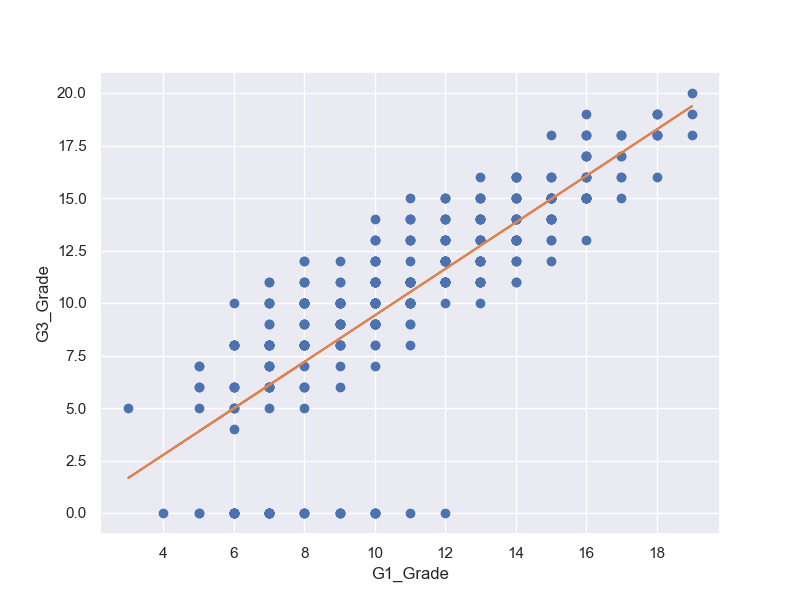
3-4-2 決定係数
R^2 = 1- \frac{\Sigma_{i=1}^{n}(y_i-f(x_i))^2}{\Sigma_{i=1}^{n}(y_i-\bar y)^2}
上式は、決定係数と呼ばれ、$R^2=1$が最大値であり、1に近ければ近いほど良いモデルになります。
print('決定係数;',reg.score(x,y))
決定係数; 0.64235084605227
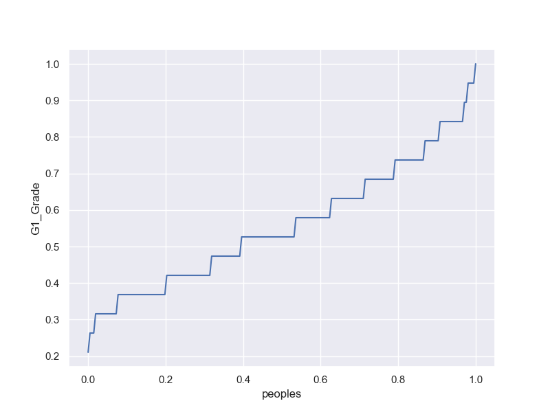
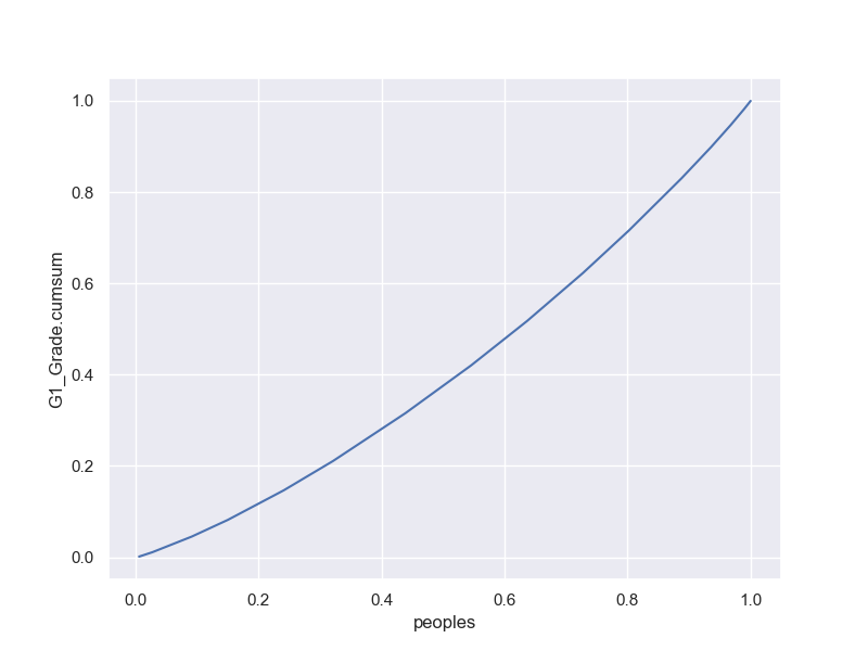
総合問題3-2-1 Lorenz Curve
df0 = student_data_math[student_data_math['sex'].isin(['M'])]
df = df0.sort_values(by=['G1'])
df['Ct']=np.arange(1,len(df)+1)

x = df['Ct']
print(x)
y = df['G1'].cumsum()
print(y)
fig, (ax1) = plt.subplots(1, 1, figsize=(8,6))
ax1.plot(x/max(x),y/max(y))
ax1.set_xlabel('peoples')
ax1.set_ylabel('G1_Grade.cumsum')
ax1.grid(True)
plt.show()

248      1
144      2
164      3
161      4
153      5
      ...
113    183
129    184
245    185
42     186
47     187
Name: Ct, Length: 187, dtype: int32
248       3
144       8
164      13
161      18
153      23
       ...
113    2026
129    2044
245    2062
42     2081
47     2100
Name: G1, Length: 187, dtype: int64
Gini係数;(0,0)(1,1)を結んだ45度直線との間の面積の2倍;不平等の度合い
M
F

参考
M;G1 vs peaples
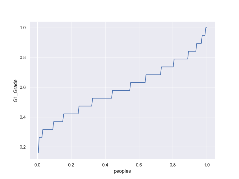
F;G1 vs peaples