Pythonを使ったデータサイエンティストになるための修行です。
ついに3種の神器のひとつPandasをやっていきましょう。
PandasはPythonの超絶最強データ解析用パッケージです。
Excelでできることはなんでもできるので非常に便利。(Excelにできないこともできる)
numpyやmatplotlibなどとの相性も抜群でシームレスに利用できる。
Pandasを使ったPythonプログラムの実行は以下で説明しているIPython Notebookを使うのが良いと思います。
PREV →【Python】蛇使いへの道 (5) Matplotlibと戯れる
NEXT → Pandasの応用(できるだけ早く)
こんな感じでDataFrameやグラフなどをキレイに可視化してくれます。すごいね。

Pandasのデータ構造
Pandasには3つのデータ構造があります。
- 1次元配列: Series
- 2次元配列: DataFrame
- 3次元配列: Panel
これらはNumpyのarrayから生成してみましょう。
Seriesの例 (1D)
Python
import numpy as np
import pandas as pd
Python
# Series
a1 = np.arange(2)
idx = pd.Index(['A', 'B'], name = 'index')
series = pd.Series(a1, index=idx)
series
index
A    0
B    1
dtype: int64
DataFrameの例 (2D)
Python
# DataFrame
a2 = np.arange(4).reshape(2, 2)
col = pd.Index(['a', 'b'], name= 'column')
df = pd.DataFrame(a2, index=idx, columns=col)
df
| column |
a |
b |
| index |
|
|
| A |
0 |
1 |
| B |
2 |
3 |
Panelの例 (3D)
Python
a3 = np.arange(8).reshape(2,2,2)
itm = pd.Index(['p', 'q'], name='item')
panel = pd.Panel(a3, items=itm, major_axis=idx, minor_axis=col)
panel['p']
| column |
a |
b |
| index |
|
|
| A |
0 |
1 |
| B |
2 |
3 |
| column |
a |
b |
| index |
|
|
| A |
4 |
5 |
| B |
6 |
7 |
2重indexを持つSeriesの例 (実質2D)
Python
a1=np.arange(4)
idx = pd.MultiIndex.from_product([['A','B'],['a','b']], names=('i','j'))
series2 = pd.Series(a1, index=idx)
series2

# 軸の多重度が3以上の場合でもfrom_productは使用できる。
# pd.MultiIndex.from_product([['A', 'B'],['a', 'b'],['1', '2']], names=('i', 'j', 'k'))
i  j
A  a    0
   b    1
B  a    2
   b    3
dtype: int64
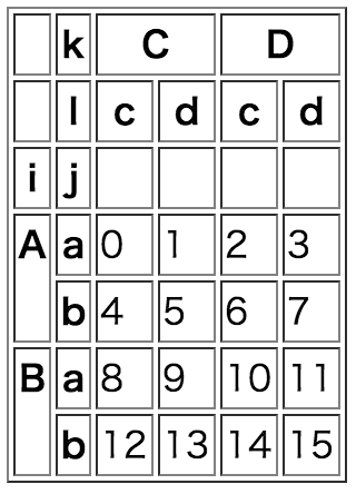
2重indexを持つDataFrameの例 (実質4D)
Python
a2 = np.arange(16) .reshape(4,4)
idx = pd.MultiIndex.from_product( [['A','B'],['a','b']], names=('i','j'))
col = pd.MultiIndex.from_product( [['C','D'],['c','d']], names=('k','l'))
df = pd.DataFrame(a2, index=idx, columns=col)
df
|
k |
C |
D |
|
l |
c |
d |
c |
d |
| i |
j |
|
|
|
|
| A |
a |
0 |
1 |
2 |
3 |
| b |
4 |
5 |
6 |
7 |
| B |
a |
8 |
9 |
10 |
11 |
| b |
12 |
13 |
14 |
15 |
今回は省略しますがPanelも同じように多重indexをもたせることができます。
データへのアクセス方法 (Indexing)
PandasとNumpyの大きな違いはPandasではNumpyのindex概念が高機能化しています。
先程の2次元配列をNumpyとPandasのDataFrameで比較してみます。
Python
a2 = np.arange(4).reshape(2, 2)
a2
Python
idx = pd.Index(['A', 'B'], name='index')
col = pd.Index(['a', 'b'], name='column')
df = pd.DataFrame(a2, index=idx, columns=col)
df
| column |
a |
b |
| index |
|
|
| A |
0 |
1 |
| B |
2 |
3 |
行にそれぞれA, B、列にa, bというラベルを付けており、Pandasではこれをindexとして利用することができます。
これはlabel-based indexと呼びます。
これに対してNumpyで使用される0から始まる整数のindexをposition-based indexと呼びます。
Pandasではこれら両方を利用可能です。
label-based indexはdictのkey的であり、position-based indexはlistのindex的であるため、Pandasはdictとlistの両方の性質を兼ね備えていると考えることもできます。
なので、もちろんNumpyと同じようにslice, fancy indexing, boolean indexingも可能です。
slice
Python
df = pd.DataFrame( np.arange(16).reshape(4, 4), index=list('ABCD'),columns=list('abcd'))
df
|
a |
b |
c |
d |
| A |
0 |
1 |
2 |
3 |
| B |
4 |
5 |
6 |
7 |
| C |
8 |
9 |
10 |
11 |
| D |
12 |
13 |
14 |
15 |
Python
# 第1行以上, 第3行未満
df.ix[1:3]
|
a |
b |
c |
d |
| B |
4 |
5 |
6 |
7 |
| C |
8 |
9 |
10 |
11 |
Python
# A行以上, C行以下
# label-based indexの場合は未満でなく以下
df.ix['A' : 'C']
|
a |
b |
c |
d |
| A |
0 |
1 |
2 |
3 |
| B |
4 |
5 |
6 |
7 |
| C |
8 |
9 |
10 |
11 |
fancy indexing
Python
# 複数行指定
df.ix[['A', 'B', 'D']]
|
a |
b |
c |
d |
| A |
0 |
1 |
2 |
3 |
| B |
4 |
5 |
6 |
7 |
| D |
12 |
13 |
14 |
15 |
|
b |
d |
| A |
1 |
3 |
| B |
5 |
7 |
| C |
9 |
11 |
| D |
13 |
15 |
boolean indexing
Python
# Trueである行を参照
df.ix[[True, False, True]]
|
a |
b |
c |
d |
| A |
0 |
1 |
2 |
3 |
| C |
8 |
9 |
10 |
11 |
Python
# Trueである列を参照
df.ix[:,[True, False, True]]
|
a |
c |
| A |
0 |
2 |
| B |
4 |
6 |
| C |
8 |
10 |
| D |
12 |
14 |
Python
# a値の2倍がc値より大きい行を参照
df.ix[df['a']*2 > df['c']]
|
a |
b |
c |
d |
| B |
4 |
5 |
6 |
7 |
| C |
8 |
9 |
10 |
11 |
| D |
12 |
13 |
14 |
15 |
軸およびindexの操作
Pandasを使う上で重要な軸の入れ替え、移動、indexのリネーム、indexのソートなどを紹介します。
軸の入れ替え (swapaxes)
Python
a2 = np.arange(4) .reshape(2, 2)
idx = pd.Index(['A', 'B'], name='index')
col = pd.Index(['a', 'b'], name='column')
df = pd.DataFrame(a2, index=idx,columns=col)
df
| column |
a |
b |
| index |
|
|
| A |
0 |
1 |
| B |
2 |
3 |
Python
# 第0軸(行)と 第1軸(列)を入れ替える
df.swapaxes(0, 1)
| index |
A |
B |
| column |
|
|
| a |
0 |
2 |
| b |
1 |
3 |
Python
# 2次元の場合は転置(T)しても同じ
df.T # transpose()の省略形
| index |
A |
B |
| column |
|
|
| a |
0 |
2 |
| b |
1 |
3 |
軸の移動 (stack / unstack)
index  column
A      a         0
       b         1
B      a         2
       b         3
dtype: int64
column  index
a       A        0
        B        2
b       A        1
        B        3
dtype: int64
Python
# stack()とunstack()は逆操作なので、この2つの操作を繰り返すと元に戻る
df.stack().unstack()
| column |
a |
b |
| index |
|
|
| A |
0 |
1 |
| B |
2 |
3 |
行が列側に移動すると、列が2重indexで表現されます。
(多重でない)DataFrameをstack() あるいは unstack()すると、 どちらも出力はSeriesとなります。
多重軸の入れ替え (swapaxes)
Python
a2 = np.arange(64).reshape(8,8)
idx = pd.MultiIndex.from_product( [['A','B'],['C','D'],['E','F']],names=list('ijk'))
col = pd.MultiIndex.from_product([['a','b'],['c','d'],['e','f']],names=list('xyz'))
df = pd.DataFrame(a2, index=idx,columns=col)
df
|
|
x |
a |
b |
|
|
y |
c |
d |
c |
d |
|
|
z |
e |
f |
e |
f |
e |
f |
e |
f |
| i |
j |
k |
|
|
|
|
|
|
|
|
| A |
C |
E |
0 |
1 |
2 |
3 |
4 |
5 |
6 |
7 |
| F |
8 |
9 |
10 |
11 |
12 |
13 |
14 |
15 |
| D |
E |
16 |
17 |
18 |
19 |
20 |
21 |
22 |
23 |
| F |
24 |
25 |
26 |
27 |
28 |
29 |
30 |
31 |
| B |
C |
E |
32 |
33 |
34 |
35 |
36 |
37 |
38 |
39 |
| F |
40 |
41 |
42 |
43 |
44 |
45 |
46 |
47 |
| D |
E |
48 |
49 |
50 |
51 |
52 |
53 |
54 |
55 |
| F |
56 |
57 |
58 |
59 |
60 |
61 |
62 |
63 |
これは各軸ともに3重(3階層)になっている例ですが、swapaxes()では、全階層まるごと入れ替えが行なわれます。
|
|
i |
A |
B |
|
|
j |
C |
D |
C |
D |
|
|
k |
E |
F |
E |
F |
E |
F |
E |
F |
| x |
y |
z |
|
|
|
|
|
|
|
|
| a |
c |
e |
0 |
8 |
16 |
24 |
32 |
40 |
48 |
56 |
| f |
1 |
9 |
17 |
25 |
33 |
41 |
49 |
57 |
| d |
e |
2 |
10 |
18 |
26 |
34 |
42 |
50 |
58 |
| f |
3 |
11 |
19 |
27 |
35 |
43 |
51 |
59 |
| b |
c |
e |
4 |
12 |
20 |
28 |
36 |
44 |
52 |
60 |
| f |
5 |
13 |
21 |
29 |
37 |
45 |
53 |
61 |
| d |
e |
6 |
14 |
22 |
30 |
38 |
46 |
54 |
62 |
| f |
7 |
15 |
23 |
31 |
39 |
47 |
55 |
63 |
多重軸の入れ替え (swaplevel / reorder_levels)
Python
# 第0軸(行)の、第0階層(i)と第2階層(z)を入れ替え
df.reorder_levels([2, 1, 0])
# swaplevel(0, 2) または swaplevel('i', 'z')でも同じ
|
|
x |
a |
b |
|
|
y |
c |
d |
c |
d |
|
|
z |
e |
f |
e |
f |
e |
f |
e |
f |
| k |
j |
i |
|
|
|
|
|
|
|
|
| E |
C |
A |
0 |
1 |
2 |
3 |
4 |
5 |
6 |
7 |
| F |
C |
A |
8 |
9 |
10 |
11 |
12 |
13 |
14 |
15 |
| E |
D |
A |
16 |
17 |
18 |
19 |
20 |
21 |
22 |
23 |
| F |
D |
A |
24 |
25 |
26 |
27 |
28 |
29 |
30 |
31 |
| E |
C |
B |
32 |
33 |
34 |
35 |
36 |
37 |
38 |
39 |
| F |
C |
B |
40 |
41 |
42 |
43 |
44 |
45 |
46 |
47 |
| E |
D |
B |
48 |
49 |
50 |
51 |
52 |
53 |
54 |
55 |
| F |
D |
B |
56 |
57 |
58 |
59 |
60 |
61 |
62 |
63 |
Python
# 第1軸(列)の、第0階層(x)と第1階層(y)を 入れ替え
df.reorder_levels([1,0,2],axis=1)
# swaplevel(0, 1, axis=1) または swaplevel('i', 'j', axis=1)でも同じ
|
|
y |
c |
d |
c |
d |
|
|
x |
a |
a |
b |
b |
|
|
z |
e |
f |
e |
f |
e |
f |
e |
f |
| i |
j |
k |
|
|
|
|
|
|
|
|
| A |
C |
E |
0 |
1 |
2 |
3 |
4 |
5 |
6 |
7 |
| F |
8 |
9 |
10 |
11 |
12 |
13 |
14 |
15 |
| D |
E |
16 |
17 |
18 |
19 |
20 |
21 |
22 |
23 |
| F |
24 |
25 |
26 |
27 |
28 |
29 |
30 |
31 |
| B |
C |
E |
32 |
33 |
34 |
35 |
36 |
37 |
38 |
39 |
| F |
40 |
41 |
42 |
43 |
44 |
45 |
46 |
47 |
| D |
E |
48 |
49 |
50 |
51 |
52 |
53 |
54 |
55 |
| F |
56 |
57 |
58 |
59 |
60 |
61 |
62 |
63 |
多重軸の移動 (stack / unstack)
stack()では列軸の最下level軸が、 行軸の最下level軸に移動します。
|
|
|
x |
a |
b |
|
|
|
y |
c |
d |
c |
d |
| i |
j |
k |
z |
|
|
|
|
| A |
C |
E |
e |
0 |
2 |
4 |
6 |
| f |
1 |
3 |
5 |
7 |
| F |
e |
8 |
10 |
12 |
14 |
| f |
9 |
11 |
13 |
15 |
| D |
E |
e |
16 |
18 |
20 |
22 |
| f |
17 |
19 |
21 |
23 |
| F |
e |
24 |
26 |
28 |
30 |
| f |
25 |
27 |
29 |
31 |
| B |
C |
E |
e |
32 |
34 |
36 |
38 |
| f |
33 |
35 |
37 |
39 |
| F |
e |
40 |
42 |
44 |
46 |
| f |
41 |
43 |
45 |
47 |
| D |
E |
e |
48 |
50 |
52 |
54 |
| f |
49 |
51 |
53 |
55 |
| F |
e |
56 |
58 |
60 |
62 |
| f |
57 |
59 |
61 |
63 |
unstack()では行軸の最下level軸が、 列軸の最下level軸に移動します。
|
x |
a |
b |
|
y |
c |
d |
c |
d |
|
z |
e |
f |
e |
f |
e |
f |
e |
f |
|
k |
E |
F |
E |
F |
E |
F |
E |
F |
E |
F |
E |
F |
E |
F |
E |
F |
| i |
j |
|
|
|
|
|
|
|
|
|
|
|
|
|
|
|
|
| A |
C |
0 |
8 |
1 |
9 |
2 |
10 |
3 |
11 |
4 |
12 |
5 |
13 |
6 |
14 |
7 |
15 |
| D |
16 |
24 |
17 |
25 |
18 |
26 |
19 |
27 |
20 |
28 |
21 |
29 |
22 |
30 |
23 |
31 |
| B |
C |
32 |
40 |
33 |
41 |
34 |
42 |
35 |
43 |
36 |
44 |
37 |
45 |
38 |
46 |
39 |
47 |
| D |
48 |
56 |
49 |
57 |
50 |
58 |
51 |
59 |
52 |
60 |
53 |
61 |
54 |
62 |
55 |
63 |
indexのrename
Python
df = pd.DataFrame( [[90, 50], [60, 80]], index=['t', 'h'],columns=['m', 'e'])
df
Python
df.index.name='名前'
df.columns.name='科目'
df.rename(index=dict(t='太郎', h='花子'), columns=dict(m='数学', e='英語'))
| 科目 |
数学 |
英語 |
| 名前 |
|
|
| 太郎 |
90 |
50 |
| 花子 |
60 |
80 |
indexでのソート
Python
df = pd.DataFrame (np.arange(9).reshape(3,3), index=['B','A','C'], columns=['c','b','a'])
df
|
c |
b |
a |
| B |
0 |
1 |
2 |
| A |
3 |
4 |
5 |
| C |
6 |
7 |
8 |
Python
# 行を行index順にソート
df.sort_index(axis=0)
|
c |
b |
a |
| A |
3 |
4 |
5 |
| B |
0 |
1 |
2 |
| C |
6 |
7 |
8 |
Python
# 列を列index順でもソート
df.sort_index(axis=0).sort_index(axis=1)
|
a |
b |
c |
| A |
5 |
4 |
3 |
| B |
2 |
1 |
0 |
| C |
8 |
7 |
6 |
データの変換
Seriesのデータ変換
Python
series=pd.Series([2, 3], index=list('ab'))
series
Python
# Seriesの各値を2乗する
series ** 2
Python
# mapで関数やdictをわたすこともできる
series.map(lambda x: x**2)
# series.map( {x:x**2 for x in range(3) })
DataFrameのデータ変換
Python
df = pd.DataFrame( [[2, 3], [4, 5]], index=list('AB'),columns=list('ab'))
df
Python
# Seriesと同様
df ** 2
# df.map(lambda x: x**2)
Python
# 関数(Series to scalar)を各列に適用する
# 次元が一つ下がり、結果はSeriesになる
df.apply(lambda c: c['A']*c['B'], axis=0)
Python
# 関数(Series to Series)を各行に適用する
# 結果はDataFrame
df.apply(lambda r: pd.Series(dict(a=r['a']+r['b'], b=r['a']*r['b'])), axis=1)
連結 (concat) と結合 (merge)
Pandasでは複数のSeriesやDataFrameの連結、結合を行うことができます。
Seriesの連結 (concat)
indexに重複があったとしてもそのまま結合されます。
Python
ser1=pd.Series([1,2], index=list('ab'))
ser2=pd.Series([3,4], index=list('bc'))
pd.concat([ser1, ser2])
a    1
b    2
b    3
c    4
dtype: int64
Python
# indexをユニークにするときは、重複inexを除いておく
dif_idx = ser2.index.difference(ser1.index)
pd.concat([ser1, ser2[list(dif_idx)]])
DataFrameの連結 (concat)
Python
df1 = pd.DataFrame([[1, 2], [3, 4]], index=list('AB'),columns=list('ab'))
df2 = pd.DataFrame([[5, 6], [7, 8]], index=list('CD'),columns=list('ab'))
df3 = pd.DataFrame([[5, 6], [7, 8]], index=list('AB'),columns=list('cd'))
Python
# 第0軸(行)方向に積み上げる
pd.concat([df1, df2], axis=0)
|
a |
b |
| A |
1 |
2 |
| B |
3 |
4 |
| C |
5 |
6 |
| D |
7 |
8 |
Python
# 第1軸(列)方向に積み上げる
pd.concat([df1, df3], axis=1)
|
a |
b |
c |
d |
| A |
1 |
2 |
5 |
6 |
| B |
3 |
4 |
7 |
8 |
DataFrameの結合 (merge)
Python
df1.index.name = df3.index.name = 'A'
df10 = df1.reset_index()
df30 = df3.reset_index()
Python
# 列Aで結合
pd.merge(df10, df30, on='A')
|
A |
a |
b |
c |
d |
| 0 |
A |
1 |
2 |
5 |
6 |
| 1 |
B |
3 |
4 |
7 |
8 |
onには結合に使用する列名を与えます。
複数指定可能でその場合はlistで与えます。
省略時には、2つDataFrameの共通列名が採用されます。
上の例では共通列名がAのみなので省略可能です。
mergeにおいては、index列は無視されるので注意が必要です。
各種ファイル形式の入出力
Pandasは色々な形式を入出力できます。
Python
a2 = np.arange(16) .reshape(4,4)
idx = pd.MultiIndex.from_product( [['A','B'],['a','b']], names=('i','j'))
col = pd.MultiIndex.from_product( [['C','D'],['c','d']], names=('k','l'))
df = pd.DataFrame(a2, index=idx, columns=col)
df
|
k |
C |
D |
|
l |
c |
d |
c |
d |
| i |
j |
|
|
|
|
| A |
a |
0 |
1 |
2 |
3 |
| b |
4 |
5 |
6 |
7 |
| B |
a |
8 |
9 |
10 |
11 |
| b |
12 |
13 |
14 |
15 |
ファイルの書き出し
Python
# HTMLファイルへの出力
df.to_html('a2.html')
Python
# Excelファイルへの出力 (openpyxlが必要)
df.to_excel('a2.xlsx')

ファイルの読み込み

Python
xl = pd.ExcelFile('test.xlsx')
# sheetの指定
df = xl.parse('Sheet1')
df
|
国語 |
数学 |
英語 |
| 太郎 |
70 |
80 |
90 |
| 花子 |
90 |
60 |
70 |
| 二郎 |
50 |
80 |
70 |
グラフの作成
PandasはMatplotlibとの相性も抜群でDataFrameからグラフを作ることも簡単にできます。
Python
%matplotlib inline

x = np.linspace(0, 2*np.pi, 10)
df = pd.DataFrame(dict(sin=np.sin(x), cos=np.cos(x)), index=x)
df
|
cos |
sin |
| 0.000000 |
1.000000 |
0.000000e+00 |
| 0.698132 |
0.766044 |
6.427876e-01 |
| 1.396263 |
0.173648 |
9.848078e-01 |
| 2.094395 |
-0.500000 |
8.660254e-01 |
| 2.792527 |
-0.939693 |
3.420201e-01 |
| 3.490659 |
-0.939693 |
-3.420201e-01 |
| 4.188790 |
-0.500000 |
-8.660254e-01 |
| 4.886922 |
0.173648 |
-9.848078e-01 |
| 5.585054 |
0.766044 |
-6.427876e-01 |
| 6.283185 |
1.000000 |
-2.449294e-16 |
