Object Detection

TORCHVISION.MODELSに用意されている RetinaNet を使用して推論を行います。
今回は物体検出の大枠の理解をゴールとします。

また Object Detection を行い、画像内に写っている車の数をカウントしたいと思います。object の数のカウントに加えて Image Classification モデルを組み合わせると、検知した車の車種を識別できたりもします。
Object Detection の目的は検知するだけでなくその後の活用方法も様々です。

import torch
import torchvision
!pip install -q pytorch_lightning
import pytorch_lightning as pl

データの準備

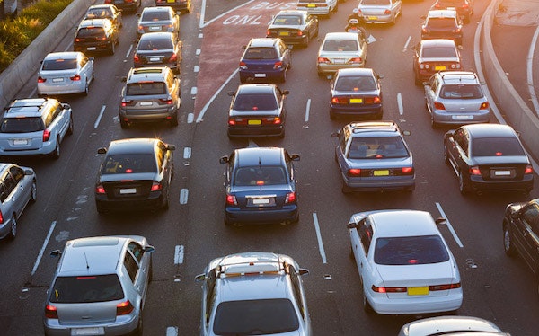
今回は画像1枚だけ推論を行います。

from torchvision import transforms
from PIL import Image
import matplotlib.pyplot as plt
img = Image.open(path)
transform = transforms.ToTensor()
x = transform(img)

モデルの用意

from torchvision.models.detection import retinanet_resnet50_fpn
# 乱数のシードを固定して再現性を確保
pl.seed_everything(0)

# RetinaNet
model = retinanet_resnet50_fpn(pretrained=True)

最初の注意点として、この retinanet_resnet50_fpn に与える引数は学習と推論で異なります。

・model.training が True
　・引数: 入力値 x と目標値 t
　・返り値: losses (RetinaNet の損失関数)
・model.training が False
　・引数: 入力値 x のみ
　・返り値
　　・boxes
　　・labels
　　・scores
初期設定では model.train が True となり学習モードとなっています。
推論結果を確認する際には model.eval() により検証モードとしておきましょう。

# 推論モードへ
model.eval()
print(model.training)

False

# 推論
y = model(x.unsqueeze(0))[0]
y

{'boxes': tensor([[365.4843, 75.9052, 426.6606, 134.5115],
[245.6993, 162.6519, 335.5136, 251.8736],
[372.4906, 133.6757, 462.0575, 215.2378],
...,
[ 91.3216, 190.7660, 187.2731, 308.8808],
[245.1367, 17.5582, 402.6794, 97.8703],
[369.6038, 115.8406, 554.9694, 364.4827]], grad_fn=<StackBackward0>),
'labels': tensor([ 3, 3, 3, 3, 3, 3, 3, 3, 3, 3, 3, 3, 3, 3, 3, 3, 3, 3,
3, 3, 3, 3, 3, 3, 3, 3, 3, 3, 8, 8, 3, 3, 8, 3, 8, 3,
8, 8, 3, 3, 3, 6, 8, 3, 8, 8, 3, 8, 3, 8, 72, 3, 3, 3,
8, 77, 10, 3, 6, 3, 3, 8, 3, 3, 3, 1, 3, 10, 3, 8, 3, 3,
3, 1, 3, 14, 8, 3, 33, 3, 3, 8, 3, 3, 14, 8, 3, 1, 3, 10,
3, 3, 3, 3, 8, 3, 33, 3, 3, 1, 3, 3, 8, 3, 1, 3, 1, 6,
3, 8, 7, 14, 3, 3, 82, 1, 3, 3, 10, 3, 3, 3, 8, 6, 1, 3,
6, 8, 10, 3, 3, 14, 3, 8, 74, 3, 1, 1, 3, 3, 1, 3, 8, 3,
8, 3, 3, 3, 8, 10, 3, 3, 1, 1, 4, 1, 33, 3, 3, 27, 5, 3,
3, 3, 3, 8, 3, 3, 3, 10, 3, 1, 3, 1, 3, 3, 3, 8, 3, 3,
3, 3, 80, 1, 3, 3, 27, 3, 3, 1, 3, 1, 35, 3, 3, 6, 3, 1,
1, 1, 4, 27, 84, 3, 8, 3, 27, 3, 10, 8, 6, 3, 10, 1, 1, 3,
3, 3, 1, 14, 3, 3, 3, 3, 3, 4, 3, 8, 3, 3, 3, 3, 27, 1,
1, 3, 3, 3, 28, 27, 8, 8, 8, 33, 1, 3, 1, 3, 3, 6, 3, 4,
4, 1, 3, 6, 8, 78, 1, 6, 3, 79, 4, 8, 8, 8, 3, 3, 3, 2]),
'scores': tensor([0.8897, 0.8844, 0.8818, 0.8809, 0.8805, 0.8797, 0.8747, 0.8654, 0.8619,
0.8598, 0.8375, 0.8251, 0.8000, 0.7942, 0.7704, 0.7447, 0.7345, 0.7210,
0.7125, 0.7097, 0.6765, 0.6685, 0.6113, 0.5613, 0.4721, 0.4537, 0.4127,
0.4013, 0.3943, 0.3350, 0.3263, 0.3192, 0.3112, 0.3066, 0.2766, 0.2766,
0.2745, 0.2718, 0.2701, 0.2645, 0.2583, 0.2574, 0.2519, 0.2503, 0.2501,
0.2432, 0.2419, 0.2417, 0.2389, 0.2379, 0.2362, 0.2298, 0.2278, 0.2265,
0.2243, 0.2223, 0.2125, 0.2098, 0.2061, 0.1972, 0.1893, 0.1824, 0.1670,
0.1647, 0.1589, 0.1587, 0.1579, 0.1564, 0.1545, 0.1526, 0.1518, 0.1487,
0.1473, 0.1472, 0.1438, 0.1419, 0.1402, 0.1395, 0.1340, 0.1328, 0.1319,
0.1282, 0.1277, 0.1252, 0.1251, 0.1229, 0.1229, 0.1223, 0.1203, 0.1199,
0.1196, 0.1188, 0.1172, 0.1155, 0.1152, 0.1145, 0.1145, 0.1141, 0.1124,
0.1119, 0.1114, 0.1107, 0.1104, 0.1078, 0.1073, 0.1071, 0.1049, 0.1045,
0.1042, 0.1030, 0.1026, 0.1025, 0.1023, 0.1019, 0.1017, 0.1003, 0.1000,
0.0990, 0.0989, 0.0985, 0.0985, 0.0973, 0.0970, 0.0964, 0.0958, 0.0956,
0.0954, 0.0951, 0.0949, 0.0947, 0.0937, 0.0932, 0.0923, 0.0922, 0.0920,
0.0919, 0.0907, 0.0906, 0.0901, 0.0900, 0.0900, 0.0893, 0.0890, 0.0889,
0.0887, 0.0873, 0.0865, 0.0860, 0.0858, 0.0858, 0.0852, 0.0848, 0.0844,
0.0843, 0.0836, 0.0834, 0.0831, 0.0827, 0.0821, 0.0818, 0.0802, 0.0800,
0.0794, 0.0793, 0.0793, 0.0788, 0.0788, 0.0787, 0.0785, 0.0784, 0.0783,
0.0781, 0.0780, 0.0777, 0.0776, 0.0775, 0.0771, 0.0762, 0.0759, 0.0758,
0.0758, 0.0756, 0.0754, 0.0753, 0.0752, 0.0752, 0.0751, 0.0747, 0.0745,
0.0745, 0.0740, 0.0740, 0.0737, 0.0735, 0.0734, 0.0731, 0.0731, 0.0730,
0.0728, 0.0728, 0.0723, 0.0722, 0.0721, 0.0719, 0.0718, 0.0715, 0.0715,
0.0711, 0.0710, 0.0708, 0.0707, 0.0706, 0.0704, 0.0702, 0.0701, 0.0699,
0.0698, 0.0691, 0.0690, 0.0689, 0.0681, 0.0680, 0.0675, 0.0674, 0.0672,
0.0670, 0.0668, 0.0668, 0.0658, 0.0657, 0.0654, 0.0651, 0.0646, 0.0634,
0.0630, 0.0627, 0.0625, 0.0618, 0.0617, 0.0613, 0.0611, 0.0608, 0.0605,
0.0601, 0.0592, 0.0591, 0.0586, 0.0583, 0.0581, 0.0577, 0.0576, 0.0576,
0.0573, 0.0570, 0.0566, 0.0566, 0.0563, 0.0558, 0.0557, 0.0556, 0.0552,
0.0550, 0.0549, 0.0545, 0.0541, 0.0537, 0.0535, 0.0532, 0.0530, 0.0520],
grad_fn=<IndexBackward0>)}

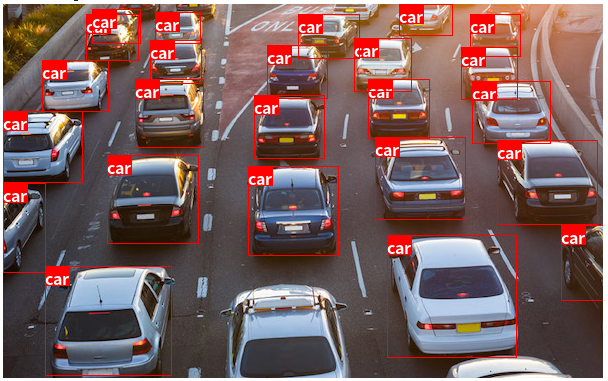
推論の結果の可視化

推論結果を可視化してみましょう。
Pillow の ImageDraw、ImageFont を使用し、ボックスとラベルを描画します。

import numpy as np
from PIL import ImageDraw, ImageFont
%%capture
!if [ ! -d fonts ]; then mkdir fonts && cd fonts && wget https://noto-website-2.storage.googleapis.com/pkgs/NotoSansCJKjp-hinted.zip && unzip NotoSansCJKjp-hinted.zip && cd .. ;fi
COCO_INSTANCE_CATEGORY_NAMES = [
    '__background__', 'person', 'bicycle', 'car', 'motorcycle', 'airplane', 'bus',
    'train', 'truck', 'boat', 'traffic light', 'fire hydrant', 'N/A', 'stop sign',
    'parking meter', 'bench', 'bird', 'cat', 'dog', 'horse', 'sheep', 'cow',
    'elephant', 'bear', 'zebra', 'giraffe', 'N/A', 'backpack', 'umbrella', 'N/A', 'N/A',
    'handbag', 'tie', 'suitcase', 'frisbee', 'skis', 'snowboard', 'sports ball',
    'kite', 'baseball bat', 'baseball glove', 'skateboard', 'surfboard', 'tennis racket',
    'bottle', 'N/A', 'wine glass', 'cup', 'fork', 'knife', 'spoon', 'bowl',
    'banana', 'apple', 'sandwich', 'orange', 'broccoli', 'carrot', 'hot dog', 'pizza',
    'donut', 'cake', 'chair', 'couch', 'potted plant', 'bed', 'N/A', 'dining table',
    'N/A', 'N/A', 'toilet', 'N/A', 'tv', 'laptop', 'mouse', 'remote', 'keyboard', 'cell phone',
    'microwave', 'oven', 'toaster', 'sink', 'refrigerator', 'N/A', 'book',
    'clock', 'vase', 'scissors', 'teddy bear', 'hair drier', 'toothbrush'
]
def visualize_results(input, output, threshold):
    image= input.permute(1, 2, 0).numpy()
    image = Image.fromarray((image*255).astype(np.uint8))

    boxes = output['boxes'].cpu().detach().numpy()
    labels = output['labels'].cpu().detach().numpy()

    if 'scores' in output.keys():
        scores = output['scores'].cpu().detach().numpy()
        boxes = boxes[scores > threshold]
        labels = labels[scores > threshold]

    draw = ImageDraw.Draw(image)
    font = ImageFont.truetype('fonts/NotoSansCJKjp-Bold.otf', 16)
    for box, label in zip(boxes, labels):
        # box
        draw.rectangle(box, outline='red')
        # label
        text = COCO_INSTANCE_CATEGORY_NAMES[label]
        w, h = font.getsize(text)
        draw.rectangle([box[0], box[1], box[0]+w, box[1]+h], fill='red')
        draw.text((box[0], box[1]), text, font=font, fill='white')

    return image
visualize_results(x, y, 0.5)

検出したObjectを切り抜き

image = Image.open(path)
threshold = 0.5

boxes = y['boxes'].cpu().detach().numpy()
labels = y['labels'].cpu().detach().numpy()
scores = y['scores'].cpu().detach().numpy()

boxes = boxes[scores > threshold]
labels = labels[scores > threshold]

objects = []

for box, label in zip(boxes, labels):
    if label == 3:
        img = image.crop(box)
        objects.append(np.array(img))

len(objects)

25

plt.figure(figsize=(10, 8))
for n, obj in enumerate(objects):
    plt.subplot(5, 5, n+1)
    plt.imshow(obj)
    plt.axis('off')

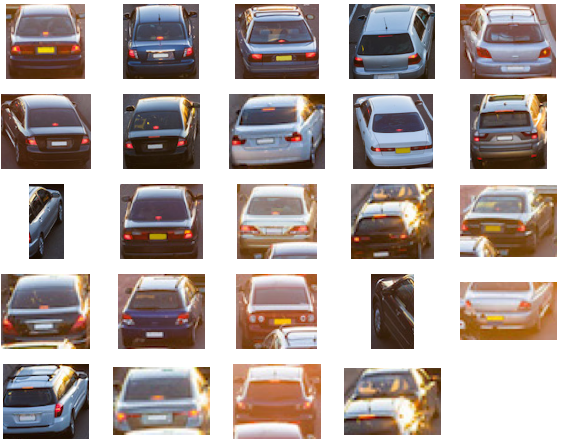
このように車のみを切り抜けています。ここから画像分類にかけて車種の判別や、台数をカウントして混雑状況を把握するなど追加のタスクを検討できます。