はじめに
最近、グラフ探索アルゴリズムについて学ぶ機会があり、なにか物理に関連付けられないかなと思ったのがこの記事を書いたきっかけです。いろいろ調べるとフェルマーの原理に応用できそうだということが分かったのでこれを自分で実装してみました。面白い結果が得られたのでぜひ最後まで読んでみてください。
フェルマーの原理とは
フェルマーの原理とは、「光は光学的距離(距離に屈折率をかけたもの)を最小にするような経路を通るという原理」です。フェルマーの原理からスネルの法則を導く手法が変分法の導入で扱われることが多く、この原理を知っている方も多いと思います。この導出の具体的方法はこの記事の本題ではないのでここでは扱いませんが知らない方はぜひ調べてみてください。
グラフについて
ここでいうグラフとは頂点と辺から成る次のような図形のことです。
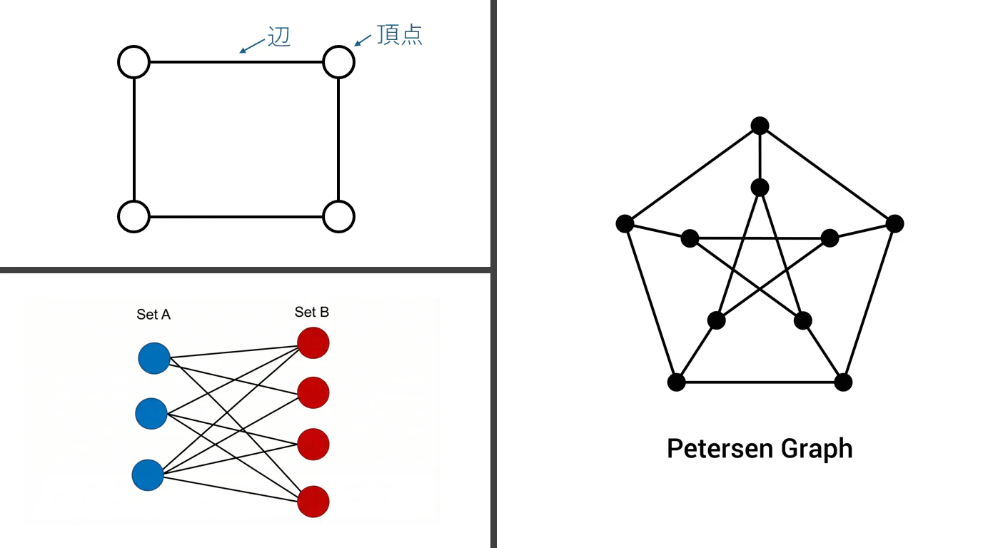
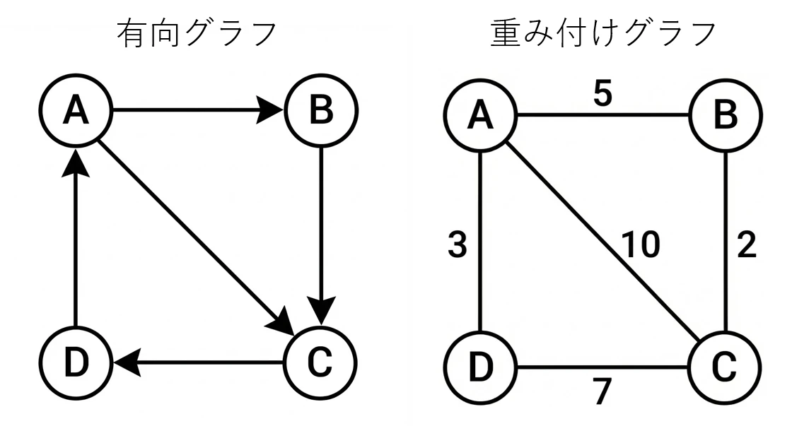
グラフにはいろいろ種類があり、例えば、各辺の通れる方向が決められている有向グラフや各辺を通るときにかかるコスト(距離など)が付された重み付きグラフなどがあります。(今回使うのは重み付き有向グラフです。)
そして、グラフ探索アルゴリズムとは特定の頂点を探したり、全体を周回するような経路を求めたりするアルゴリズムのことです。代表的なものにBFS(幅優先探索)やDFS(深さ優先探索)などがあります。ここでは詳しくは書かないので興味があれば調べてみてください。
ダイクストラ法
ダイクストラ法は重み付きグラフのある頂点から別の頂点までの経路でコストを最小にするものを求めるのに便利なアルゴリズムです。ただしコストが負の辺がある場合は使えません。ダイクストラ法のアルゴリズムを具体例を用いて説明します。
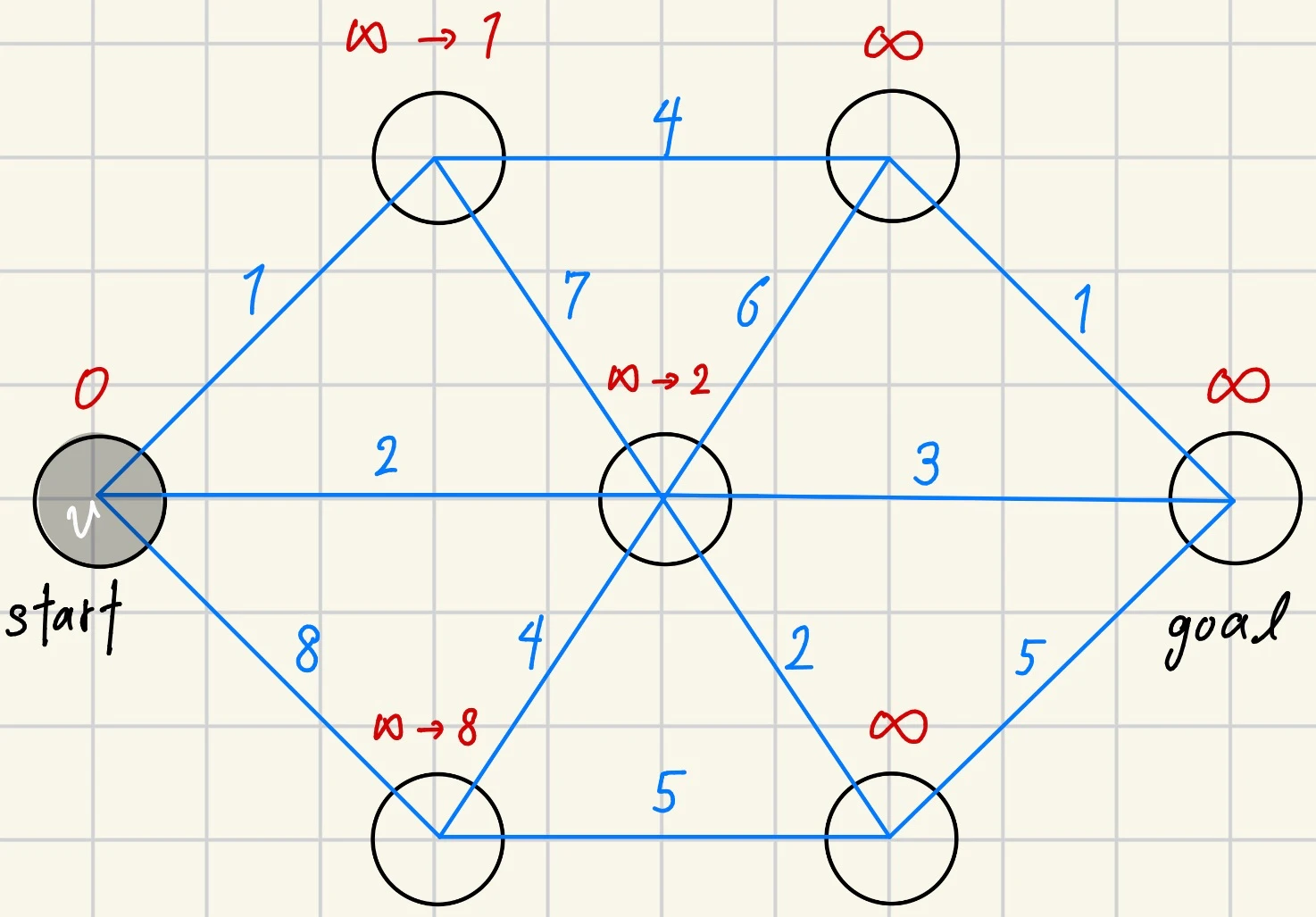
次のような重み付きグラフを考えます。始点のコストを0、それ以外の頂点のコストを∞に設定しておきます。
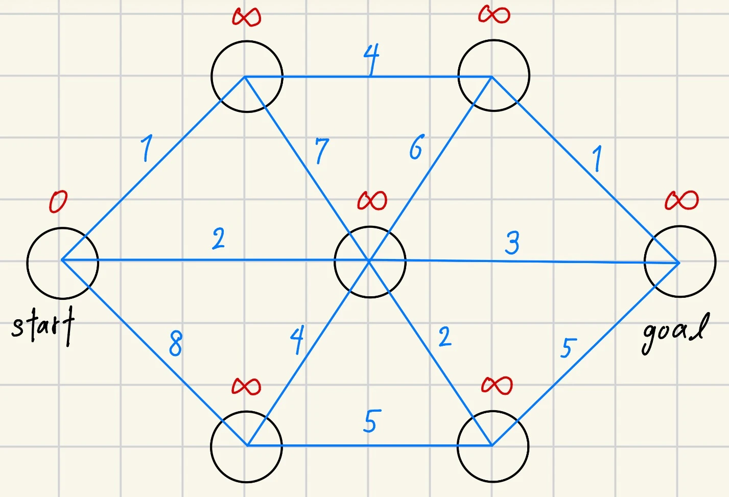
・step1 スタートの頂点を$v$として、これを塗りつぶします。
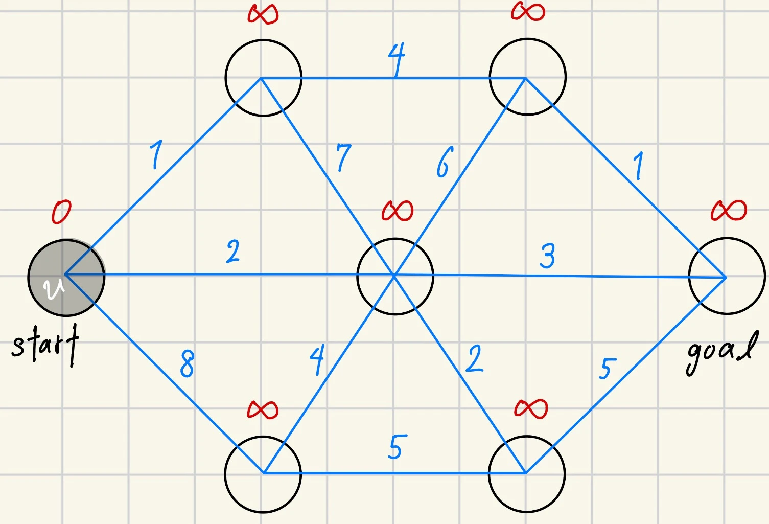
・step2 $v$に隣接するまだ塗りつぶされていない頂点について、そのコストを$min($現在のコスト$,v$のコスト+辺のコスト$)$に更新します。
・step3 まだ塗りつぶされていない頂点のうちコストが一番小さいものを選び、これを新しく$v$としたあと、これを塗りつぶします。その後、step2に戻ります。
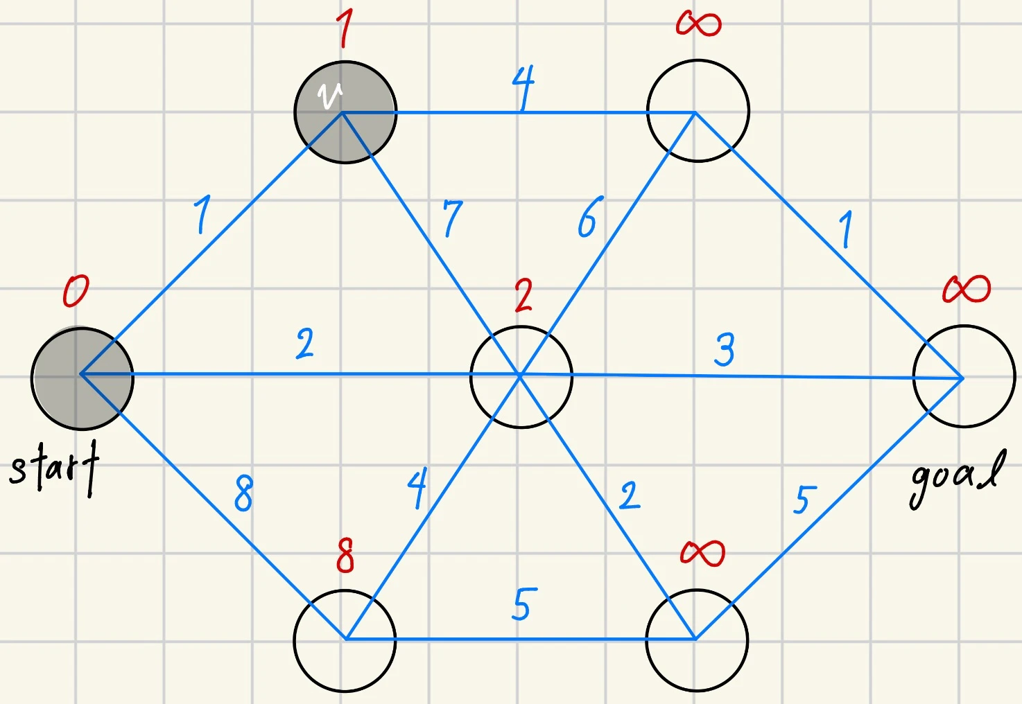
step2、step3はゴールの頂点が塗りつぶされるまで繰り返します。
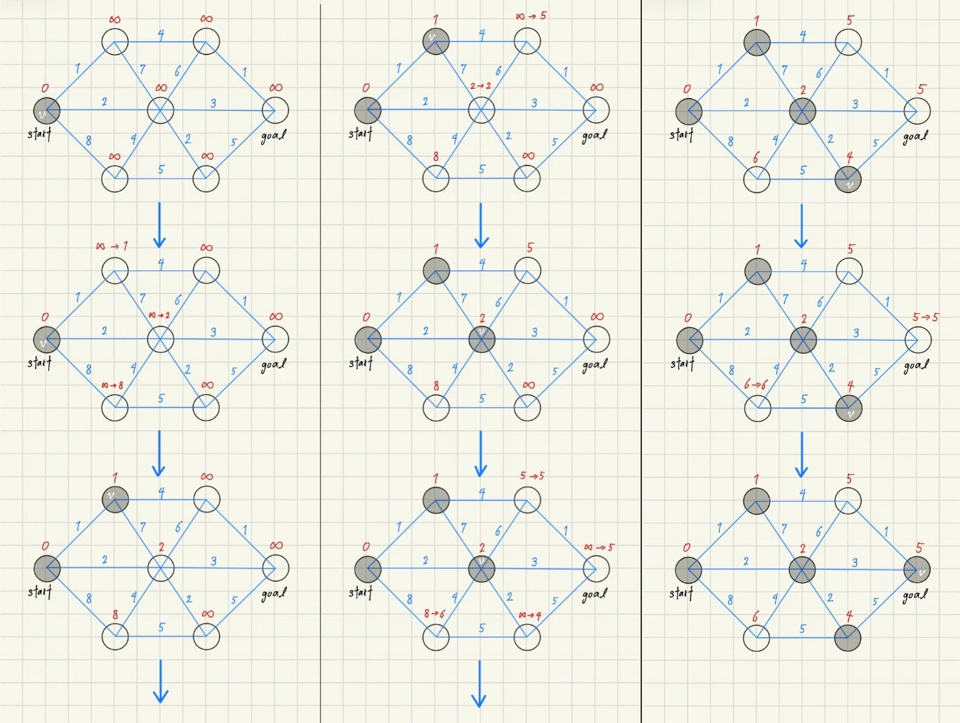
これが終了したときのゴールのコストが、スタートからゴールに行くときの最小コストになっています。この例の場合は5になりました。
最小光路探索の実装
フェルマーの原理をダイクストラ法で解くアルゴリズムをPythonで実装していきます。コードの全体は一番最後に載せます。プログラミングは初心者なので不備があるかもしれません。その場合の指摘やアドバイスなどはコメントで教えていただけるとありがたいです。あと、コードがとても読みづらいと思います。すみません...
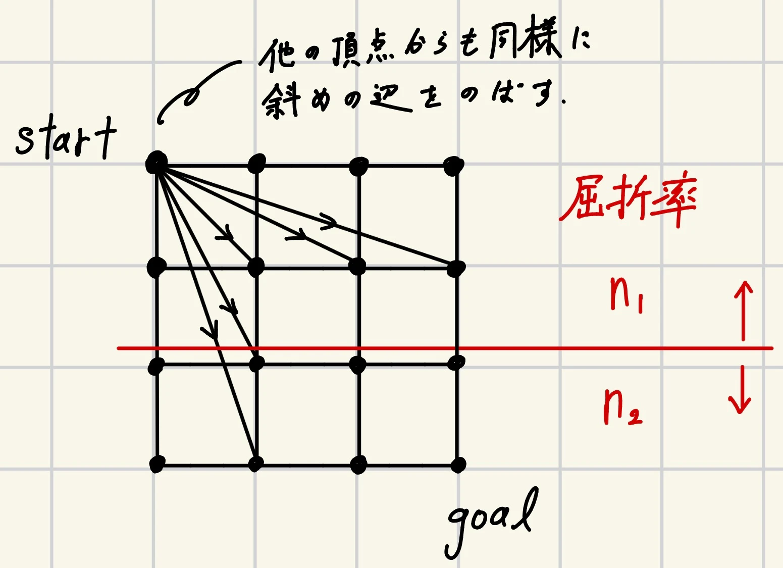
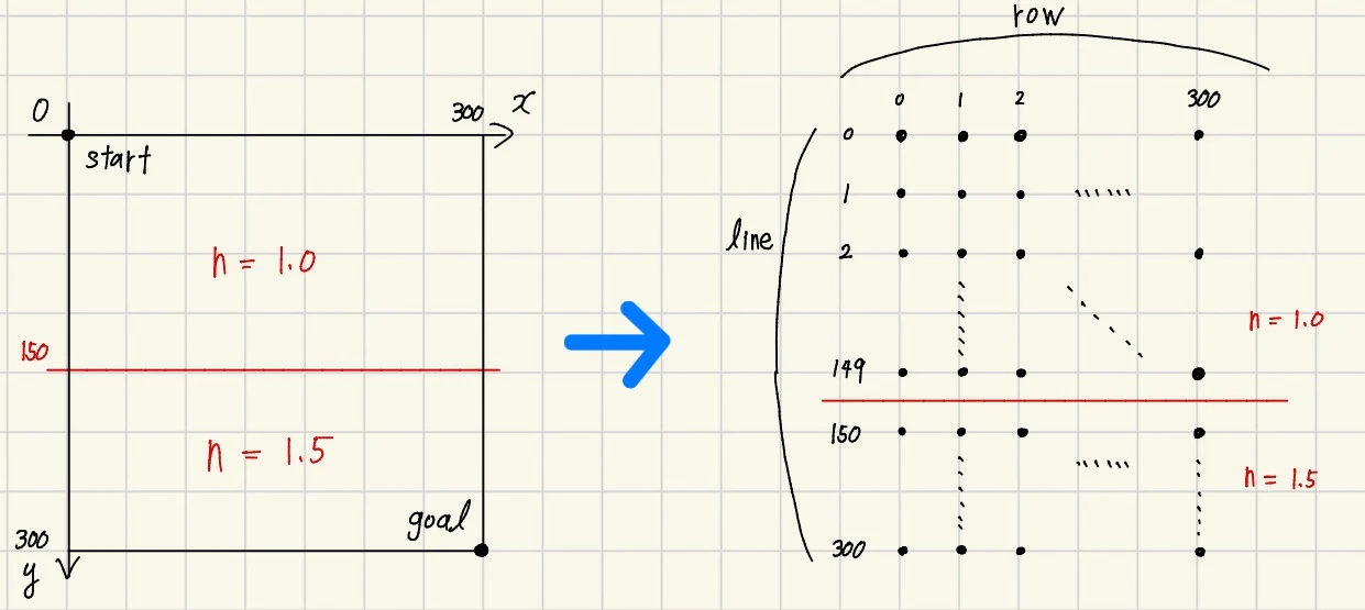
簡単に説明すると下図のようなメッシュを張って、各辺のコストは光学的距離とします。このグラフをダイクストラ法を用いて始点から終点まで最小のコストでいけるような経路を探索しています。
詳しく説明していきます。
・グラフの作成
ここでは300×300のメッシュを使います。
まず、屈折率を次のように設定します。
#屈折率
def refractive_index(line, row):
    boundary=[0, 150] #0は入れる,300(N_line)は入れない
    n=[1.0, 1.5]
    for i in range(len(boundary)-1):
        if boundary[i]<=line<boundary[i+1]:
            return n[i], boundary, n
    return n[-1], boundary, n
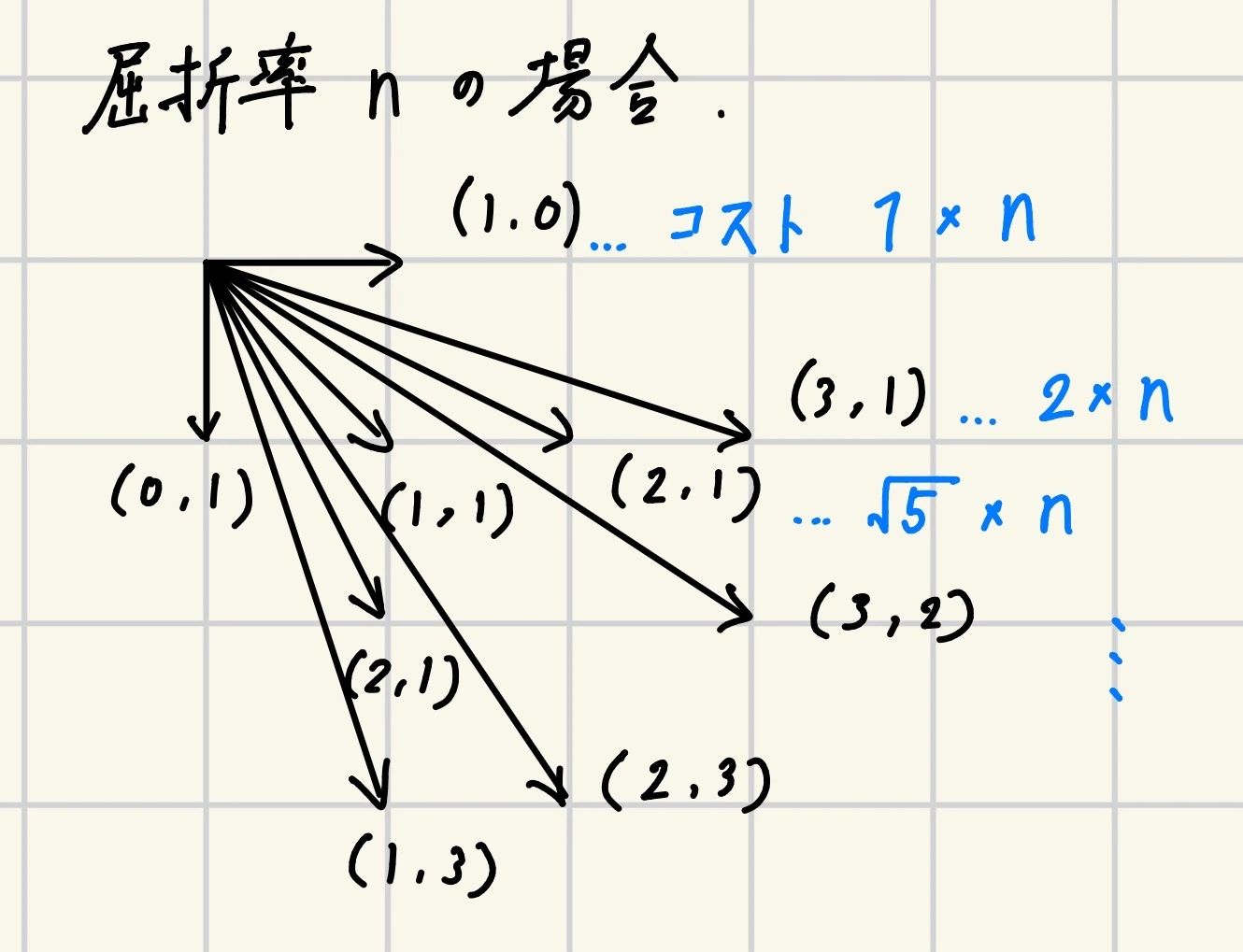
次にグラフを作成します。辺の方向は右下に伸びるように21種類の角度のものを用意しました。計算結果の精度を上げたい場合、これを増やすことで可能です。
すべての辺について始点、終点とコスト(光学的距離)を配列で記録していきます。
#頂点(line, row)の配列上での位置
def locate(line, row):
    return N_row*line+row

inf=float("INF")

#重み付き有向グラフ
N_line=301
N_row=301
N_node=N_line*N_row
list_edge = [
    (1,0), (0,1),
    (1,1),
    (2,1), (1,2),
    (3,1), (1,3),
    (3,2), (2,3),
    (4,1), (1,4),
    (4,3), (3,4),
    (5,1), (1,5),
    (5,2), (2,5),
    (5,3), (3,5),
    (5,4), (4,5)
] #辺の方向
gragh=[[] for _ in range(N_node)] #隣接リスト[辺の始点(N_node)][(辺の終点,光学的距離),...]
for node in range(N_node): #すべての頂点について
    line=node//N_row
    row=node%N_row
    for edge in list_edge: #list_edgeにある辺を追加
        dx=edge[0]
        dy=edge[1]
        terminal=locate(line+dy, row+dx)
        if line+dy<N_line and row+dx<N_row: #(N_line)×(N_row)を超えない範囲で
            actual_distance=np.sqrt(dx**2+dy**2)
            refractive=refractive_index(line, row)
            optical_distance=actual_distance*refractive[0] #光路長=距離×屈折率
            gragh[node].append([terminal, optical_distance])
これでグラフの作成が完了しました。
・ダイクストラ法の実装
前に説明したダイクストラ法を頑張って実装します。ここが一番苦労しました。
#最短経路探索(ダイクストラ法)
def dijkstra(gragh, start, end): #graghの頂点startからendまでの最短経路をもとめるダイクストラ法
#-----step1-----
    cost=[inf]*len(gragh) #各頂点までの最小光路長
    visit=[0]*len(gragh) #startからの最短経路未探索は0,探索済みは1
    path_data=[-1]*len(gragh)#経路復元用(termまでの最適経路のtermの1つ前の頂点を記録)
    cost[start]=0 #sart地点までの(光学的)距離0
    heap=[(0, start)] #起点選択用優先度つきキュー
    search=start #起点

    while visit[end]==0: #endに達するまで繰り返し
#-----step2-----
        for i in range(len(gragh[search])): #頂点iからのびるすべての辺について
            term=gragh[search][i][0] #辺の終点
            dist=gragh[search][i][1] #辺のコスト
            if cost[term]>cost[search]+dist: #古いコスト>新しいコストなら
                cost[term]=cost[search]+dist #コストを更新
                path_data[term]=search #経路を記録(termまでの最適経路のtermの1つ前の頂点を記録)
                heapq.heappush(heap, (cost[term], term)) #次の起点の候補に追加
        visit[search]=1 #searchは探索済み
#-----step3-----
        if heap==[]: #次の候補が空ならブレーク
            break
        while heap:
            a=heapq.heappop(heap) #heapからコスト最小のものを取り出す
            if visit[a[1]]==1: #選んだものの頂点が探索済みならcontinue(選びなおす)
                continue
            else: #探索済みならこれを次の起点にする
                search=a[1]
                break

    print(cost[end])
    return path_data
・経路の復元
上のダイクストラ法で始点から終点までの光学的距離の最小値は分かりました。しかし、このときどの経路を通ったのかを記録できていません。そこで、その経路を復元しようというのがここでやっていることです。
経路は終点から復元していきます。ダイクストラ法のアルゴリズムを見てもらえば分かるように、始点からある頂点までの最適経路のうちその頂点の1つ前に通る頂点を記録しておくことができます。(この操作はダイクストラ法の実装のところのコードに入っています。)これを使って、終点から1つずつ戻っていくことを繰り返せば全体の経路を復元できるというわけです。
#経路復元
def path_restore(path): #経路を終点から復元
    path_x=[]
    path_y=[]
    i=N_node-1
    while i>=0:
        x=i%N_row
        y=i//N_row
        path_x.append(x)
        path_y.append(y)
        i=path[i]
    return(path_x, path_y)
・図の作成
光の通ってきた経路を可視化します。matplotlibの使い方を知っていればここは苦労しないと思います。
def plot(x, y, boundary, n):
    plt.figure()
    plt.gca().invert_yaxis()
    for i in boundary[1:len(boundary)]:
        plt.axhline(y=i+0.5, color="red", linestyle="--")
    boundary.append(N_line)
    for i in range(len(boundary)-1):
        plt.text(N_row*9//10, (boundary[i]+boundary[i+1])//2, "n="+str(n[i]), color="red")
    plt.plot(x, y, marker=".", markersize=2, label="Light Path")
    plt.title("Fermat's Principle")
    plt.legend()
    plt.grid()
    plt.show()
これで実装は完了しました。コードの全体は一番最後に載せています。
結果
実行結果を見ていきましょう!
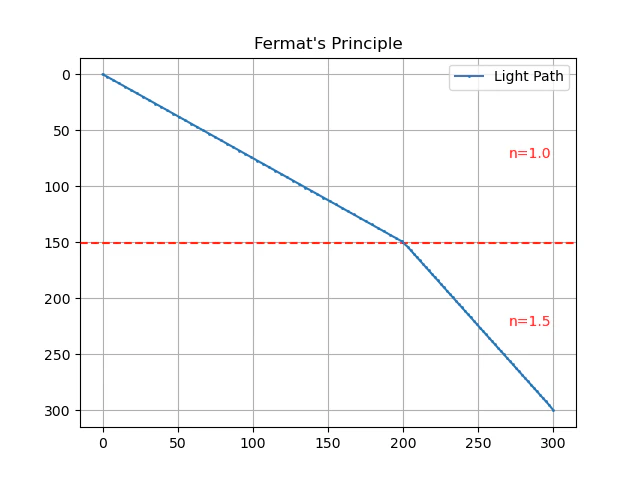
屈折率が変わる境界できれいに折れ曲がっています。光の屈折がちゃんと再現できていますね。
屈折率の設定をいじって条件を変えることもできます。複数の境界を作ってみました。
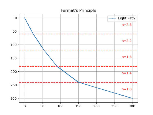
こちらもきれいに光の経路が求まりましたね。屈折率のところの関数をいじるだけで簡単にできるので皆さんもいろいろな条件を試してみてください!
以上です。ありがとうございました!
ソースコード
1つ目のやつ(境界が1つ)
import numpy as np
import heapq
import matplotlib.pyplot as plt
plt.rcParams["backend"]="qtagg"

#屈折率
def refractive_index(line, row):
    boundary=[0, 150] #0は入れる,300(N_line)は入れない
    n=[1.0, 1.5]
    for i in range(len(boundary)-1):
        if boundary[i]<=line<boundary[i+1]:
            return n[i], boundary, n
    return n[-1], boundary, n


#頂点(line, row)の配列上での位置
def locate(line, row):
    return N_row*line+row

inf=float("INF")

#重み付き有向グラフ
N_line=301
N_row=301
N_node=N_line*N_row
list_edge = [
    (1,0), (0,1),
    (1,1),
    (2,1), (1,2),
    (3,1), (1,3),
    (3,2), (2,3),
    (4,1), (1,4),
    (4,3), (3,4),
    (5,1), (1,5),
    (5,2), (2,5),
    (5,3), (3,5),
    (5,4), (4,5)
] #辺の方向
gragh=[[] for _ in range(N_node)] #隣接リスト[辺の始点(N_node)][(辺の終点,光学的距離),...]
for node in range(N_node): #すべての頂点について
    line=node//N_row
    row=node%N_row
    for edge in list_edge: #list_edgeにある辺を追加
        dx=edge[0]
        dy=edge[1]
        terminal=locate(line+dy, row+dx)
        if line+dy<N_line and row+dx<N_row: #(N_line)×(N_row)を超えない範囲で
            actual_distance=np.sqrt(dx**2+dy**2)
            refractive=refractive_index(line, row)
            optical_distance=actual_distance*refractive[0] #光路長=距離×屈折率
            gragh[node].append([terminal, optical_distance])

#最短経路探索(ダイクストラ法)
def dijkstra(gragh, start, end): #graghの頂点startからendまでの最短経路をもとめるダイクストラ法
#-----step1-----
    cost=[inf]*len(gragh) #各頂点までの最小光路長
    visit=[0]*len(gragh) #startからの最短経路未探索は0,探索済みは1
    path_data=[-1]*len(gragh)#経路復元用(termまでの最適経路のtermの1つ前の頂点を記録)
    cost[start]=0 #sart地点までの(光学的)距離0
    heap=[(0, start)] #起点選択用優先度つきキュー
    search=start #起点

    while visit[end]==0: #endに達するまで繰り返し
#-----step2-----
        for i in range(len(gragh[search])): #頂点iからのびるすべての辺について
            term=gragh[search][i][0] #辺の終点
            dist=gragh[search][i][1] #辺のコスト
            if cost[term]>cost[search]+dist: #古いコスト>新しいコストなら
                cost[term]=cost[search]+dist #コストを更新
                path_data[term]=search #経路を記録(termまでの最適経路のtermの1つ前の頂点を記録)
                heapq.heappush(heap, (cost[term], term)) #次の起点の候補に追加
        visit[search]=1 #searchは探索済み
#-----step3-----
        if heap==[]: #次の候補が空ならブレーク
            break
        while heap:
            a=heapq.heappop(heap) #heapからコスト最小のものを取り出す
            if visit[a[1]]==1: #選んだものの頂点が探索済みならcontinue(選びなおす)
                continue
            else: #探索済みならこれを次の起点にする
                search=a[1]
                break

    print(cost[end])
    return path_data

#経路復元
def path_restore(path): #経路を終点から復元
    path_x=[]
    path_y=[]
    i=N_node-1
    while i>=0:
        x=i%N_row
        y=i//N_row
        path_x.append(x)
        path_y.append(y)
        i=path[i]
    return(path_x, path_y)

#図をプロット
def plot(x, y, boundary, n):
    plt.figure()
    plt.gca().invert_yaxis()
    for i in boundary[1:len(boundary)]:
        plt.axhline(y=i+0.5, color="red", linestyle="--")
    boundary.append(N_line)
    for i in range(len(boundary)-1):
        plt.text(N_row*9//10, (boundary[i]+boundary[i+1])//2, "n="+str(n[i]), color="red")
    plt.plot(x, y, marker=".", markersize=2, label="Light Path")
    plt.title("Fermat's Principle")
    plt.legend()
    plt.grid()
    plt.show()

path=dijkstra(gragh, 0, N_node-1)
x, y=path_restore(path)
plot(x, y, boundary=refractive_index(0,0)[1], n=refractive_index(0,0)[2])
2つ目のやつ(境界が複数) #屈折率のところ以外はすべて上と同じです。
import numpy as np
import heapq
import matplotlib.pyplot as plt
plt.rcParams["backend"]="qtagg"

#屈折率
def refractive_index(line, row):
    boundary=[0, 60, 120, 180, 240] #0は入れる,300(N_line)は入れない
    n=[2.6, 2.2, 1.8, 1.4, 1.0]
    for i in range(len(boundary)-1):
        if boundary[i]<=line<boundary[i+1]:
            return n[i], boundary, n
    return n[-1], boundary, n


#頂点(line, row)の配列上での位置
def locate(line, row):
    return N_row*line+row

inf=float("INF")

#重み付き有向グラフ
N_line=301
N_row=301
N_node=N_line*N_row
list_edge = [
    (1,0), (0,1),
    (1,1),
    (2,1), (1,2),
    (3,1), (1,3),
    (3,2), (2,3),
    (4,1), (1,4),
    (4,3), (3,4),
    (5,1), (1,5),
    (5,2), (2,5),
    (5,3), (3,5),
    (5,4), (4,5)
] #辺の方向
gragh=[[] for _ in range(N_node)] #隣接リスト[辺の始点(N_node)][(辺の終点,光学的距離),...]
for node in range(N_node): #すべての頂点について
    line=node//N_row
    row=node%N_row
    for edge in list_edge: #list_edgeにある辺を追加
        dx=edge[0]
        dy=edge[1]
        terminal=locate(line+dy, row+dx)
        if line+dy<N_line and row+dx<N_row: #(N_line)×(N_row)を超えない範囲で
            actual_distance=np.sqrt(dx**2+dy**2)
            refractive=refractive_index(line, row)
            optical_distance=actual_distance*refractive[0] #光路長=距離×屈折率
            gragh[node].append([terminal, optical_distance])

#最短経路探索(ダイクストラ法)
def dijkstra(gragh, start, end): #graghの頂点startからendまでの最短経路をもとめるダイクストラ法
#-----step1-----
    cost=[inf]*len(gragh) #各頂点までの最小光路長
    visit=[0]*len(gragh) #startからの最短経路未探索は0,探索済みは1
    path_data=[-1]*len(gragh)#経路復元用(termまでの最適経路のtermの1つ前の頂点を記録)
    cost[start]=0 #sart地点までの(光学的)距離0
    heap=[(0, start)] #起点選択用優先度つきキュー
    search=start #起点

    while visit[end]==0: #endに達するまで繰り返し
#-----step2-----
        for i in range(len(gragh[search])): #頂点iからのびるすべての辺について
            term=gragh[search][i][0] #辺の終点
            dist=gragh[search][i][1] #辺のコスト
            if cost[term]>cost[search]+dist: #古いコスト>新しいコストなら
                cost[term]=cost[search]+dist #コストを更新
                path_data[term]=search #経路を記録(termまでの最適経路のtermの1つ前の頂点を記録)
                heapq.heappush(heap, (cost[term], term)) #次の起点の候補に追加
        visit[search]=1 #searchは探索済み
#-----step3-----
        if heap==[]: #次の候補が空ならブレーク
            break
        while heap:
            a=heapq.heappop(heap) #heapからコスト最小のものを取り出す
            if visit[a[1]]==1: #選んだものの頂点が探索済みならcontinue(選びなおす)
                continue
            else: #探索済みならこれを次の起点にする
                search=a[1]
                break

    print(cost[end])
    return path_data

#経路復元
def path_restore(path): #経路を終点から復元
    path_x=[]
    path_y=[]
    i=N_node-1
    while i>=0:
        x=i%N_row
        y=i//N_row
        path_x.append(x)
        path_y.append(y)
        i=path[i]
    return(path_x, path_y)

#図をプロット
def plot(x, y, boundary, n):
    plt.figure()
    plt.gca().invert_yaxis()
    for i in boundary[1:len(boundary)]:
        plt.axhline(y=i+0.5, color="red", linestyle="--")
    boundary.append(N_line)
    for i in range(len(boundary)-1):
        plt.text(N_row*9//10, (boundary[i]+boundary[i+1])//2, "n="+str(n[i]), color="red")
    plt.plot(x, y, marker=".", markersize=2, label="Light Path")
    plt.title("Fermat's Principle")
    plt.legend()
    plt.grid()
    plt.show()

path=dijkstra(gragh, 0, N_node-1)
x, y=path_restore(path)
plot(x, y, boundary=refractive_index(0,0)[1], n=refractive_index(0,0)[2])