10年前、講義で簡単なシミュレーションと考察をする課題が出たとき、ヘルプを求めた研究室の先輩から「お前は制御系の研究室にいる癖にシミュレーションのひとつも組めねえのか!?」と怒られた自分を供養します。
この記事って?
下記みたいなニッチな要望をお持ちの方へ、サンプルを組んでみました
- ちゃちゃっとシミュレーションを組みたい
- でもExcelで組むには少し複雑…
- かといってSimulinkでモデルを組むのはやったことない…
- プログラミングの経験自体はあるから、できればスクリプトで組みたい
- あわよくば「MATLABですか?少々嗜んだくらいですよ」って、できるやつ感を醸しだしたい
ただforループをぶん回すだけだと"できるやつ感"が薄いので、ode45を使用します。
ode45ってなんじゃ?という方は下記リンクをご覧ください。非常にわかりやすくまとめられております。
問題設定
やはり制御の基本問題と言ったらばねマスダンパ系でしょう(諸説あり)。
※本章の記載はこちらの記事から引用させていただきました

\left[
\begin{array}{c}
      \dot{x}_1 \\
      \dot{x}_2
    \end{array}
  \right]
=\left[
    \begin{array}{cc}
      0 & 1  \\
      -\frac{k}{m} & -\frac{c}{m}
    \end{array}
  \right]
  \left[
    \begin{array}{c}
      x_1 \\
      x_2
    \end{array}
  \right]
+ \left[
    \begin{array}{c}
      0 \\
      \frac{1}{m}
    \end{array}
  \right] u
\dot{\boldsymbol{x}}
=\left[
    \begin{array}{cc}
      0 & 1  \\
      -\frac{k}{m} & -\frac{c}{m}
    \end{array}
  \right]
\boldsymbol{x} + \left[
    \begin{array}{c}
      0 \\
      \frac{1}{m}
    \end{array}
  \right] u
$$\dot{\boldsymbol{x}}
=\boldsymbol{A}\boldsymbol{x} + \boldsymbol{B} u$$
※不要な補足かもしれませんが、$x_1$が位置、$x_2$が速度、$u$が力です。
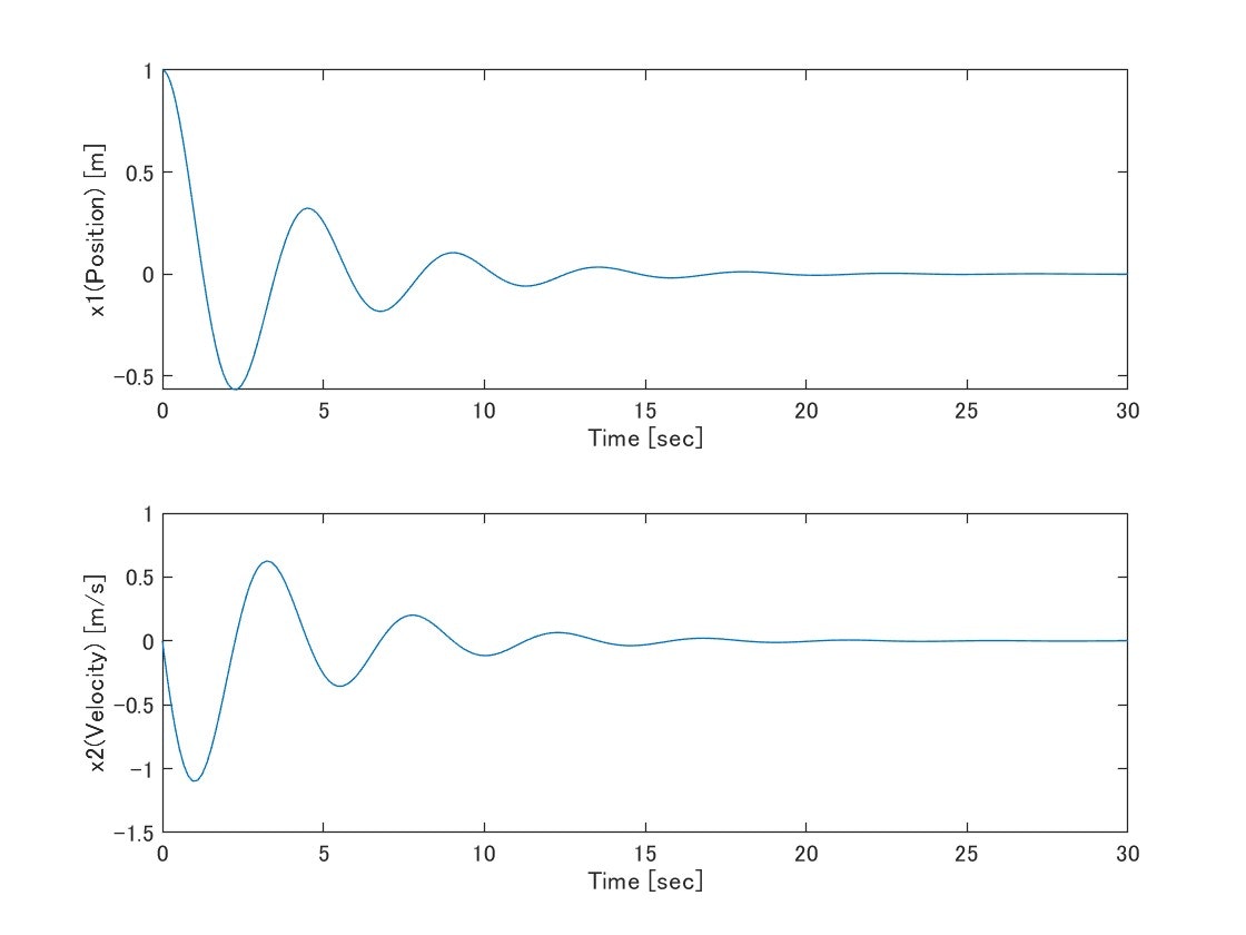
自由応答(固定値入力)のシミュレーション
一番シンプルな形がこちら。状態方程式を記載してode45をぶん回すだけです。すごくシンプルな反面、制御則については記載ができていません。これでは固定値の入力しかシミュレーションできませんね。
% Initialize
tSpan = [0 30];
x0 = [1 0]';
u = 0;

m = 1;
k = 2;
c = 0.5;

A = [0 1;
     -k/m -c/m];
B = [0;
     1/m];

% Simulation
[t,x] = ode45(@(t,x) A*x + B*u, tSpan, x0);

% Plot
figure
subplot(2,1,1)
plot(t,x(:,1))
xlabel("Time [sec]");
ylabel("x1(Position) [m]");
subplot(2,1,2)
plot(t,x(:,2))
xlabel("Time [sec]");
ylabel("x2(Velocity) [m/s]");
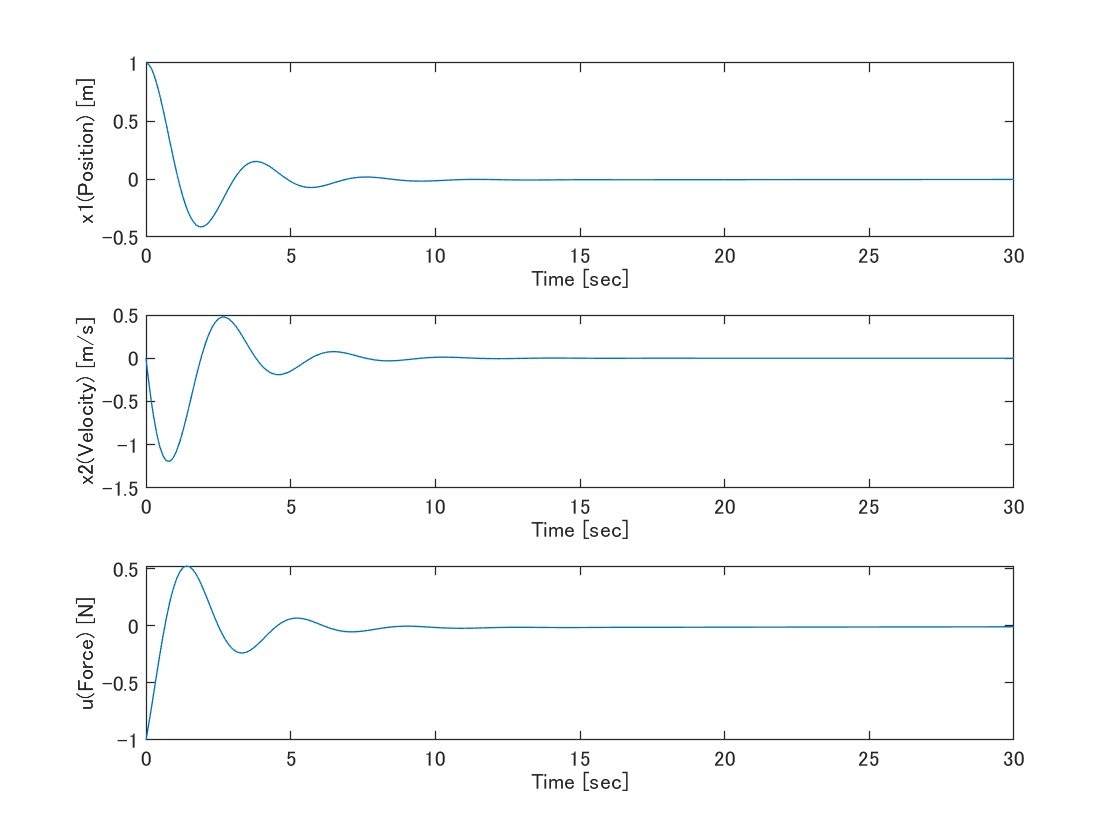
PID制御
PID制御を導入した姿がこちら。簡単化のために目標値は0にしています。
ダイナミクスの記述に変更があり、積分誤差を仮想状態として追加しています。これにより、PIDに使用する誤差(位置)/積分された誤差/誤差の微分(速度)がそれぞれ状態量として表現されるため、PIDのゲインをまとめたベクトルと状態ベクトルで内積を取れば、それがPIDとしての入力になります。
積分誤差が状態になるなら、その微分方程式である状態方程式としては積分されていない誤差そのものが記述されます。
\left[
\begin{array}{c}
      \dot{x}_1 \\
      \dot{x}_2 \\
      \dot{e}
    \end{array}
  \right]
=\left[
    \begin{array}{cc}
      0 & 1 & 0  \\
      -\frac{k}{m} & -\frac{c}{m} & 0 \\
      1 & 0 & 0
    \end{array}
  \right]
  \left[
    \begin{array}{c}
      x_1 \\
      x_2 \\
      e
    \end{array}
  \right]
+ \left[
    \begin{array}{c}
      0 \\
      \frac{1}{m} \\
      0
    \end{array}
  \right] u
※これまた不要な補足かもしれませんが、$x_1$が位置、$x_2$が速度、$e$が積分誤差、$u$が力です。
% Initialize
tSpan = [0 30];
x0 = [1 0 0]'; %誤差積分用の拡張

m = 1;
k = 2;
c = 0.5;

A = [0 1 0;
     -k/m -c/m 0;
     1 0 0];
B = [0;
     1/m;
     0];

Kp = 1;
Ki = 0.1;
Kd = 0.5;

% Simulation
[t,x] = ode45(@(t,x) myDynamics(t,x,A,B,Kp,Ki,Kd), tSpan, x0);

%ode45では入力uの時系列が保存されないので、Plot用にt,xを使用してuをReSimする
u = x * -[Kp Kd Ki]';

% Plot
figure
subplot(3,1,1)
plot(t,x(:,1))
xlabel("Time [sec]");
ylabel("x1(Position) [m]");
subplot(3,1,2)
plot(t,x(:,2))
xlabel("Time [sec]");
ylabel("x2(Velocity) [m/s]");
subplot(3,1,3)
plot(t,u(:,1))
xlabel("Time [sec]");
ylabel("u(Force) [N]");

% Local Function
function dxdt = myDynamics(t,x,A,B,Kp,Ki,Kd)

    %Controller
    u = -[Kp Kd Ki] * x;

    %State Update
    dxdt = A*x + B*u;

end
余談
正直、PIDレベルであれば上述した例でも問題はない気がするのですが、もう少し突き詰めます。ここまで来ると当初の目的から逸脱してただの興味です。ご容赦ください。
さて、先ほどの例では、uをode45実行後に改めて計算してplot用の配列を作成しています。これはode45の出力がt, xのみで、uが出力になっていないためです。別に問題ないっちゃないのですが、実際にシミュレーションの過程でどんな入力になっているかという値にはなっておりません。
ここら辺をどうにかできないか 頑張ってみます 頑張ってみました。
ode45のoutputFcnを使って毎時刻におけるuを配列に追加しています。ローカル関数内でuLogにアクセスするために、入れ子関数の形態をとっています。
% Initialize
tSpan = [0 30];
x0 = [1 0 0]'; %誤差積分用の拡張
u0 = 0;

dynamicsFunc = @myDynamics;
ctrlFunc = @myController;

% Simulation
[t, x, u] = mySimulation(dynamicsFunc, ctrlFunc, x0, u0, tSpan);

% Plot
figure
subplot(3,1,1)
plot(t,x(:,1))
subplot(3,1,2)
plot(t,x(:,2))
subplot(3,1,3)
plot(t,u(:,1))

% Local Function
function dxdt = myDynamics(t,x,u)

    % Initialize
    m = 1;
    k = 2;
    c = 0.5;

    A = [0 1 0;
         -k/m -c/m 0;
         1 0 0];
    B = [0;
         1/m;
         0];

    % State Update
    dxdt = A*x + B*u;

end

function u = myController(t,x,u0)

    % Initialize
    u = u0;
    Kp = 1;
    Ki = 0.1;
    Kd = 0.5;

    % Calculate Input
    u = -[Kp Kd Ki] * x;

end
function [tLog, xLog, uLog] = mySimulation(dynamicsFunc, ctrlFunc, x0, u0, tSpan)

    options = odeset('OutputFcn', @(t,x,flag) outputFcn(t,x,flag, u0));

    [tLog, xLog] = ode45(@(t,x) mySystem(t,x,u0), tSpan, x0, options);

    % Local Function
    function dxdt = mySystem(t,x,u0)

        % Controller
        u = ctrlFunc(t,x,u0);

        % State update
        dxdt = dynamicsFunc(t,x,u);

    end

    function status = outputFcn(t, x, flag, u0)
        status = 0;

        switch flag
            case 'init'
                uLog = u0;
            case ''
                for i = 1:length(t)
                    u = ctrlFunc(t,x(:,i),u0);
                    uLog(end+1,1) = u;
                end
            case 'done'
                %
        end
    end
end
