BRRのギブスサンプリングによるパラメータ推定②実装編 #R

Bayesian Ridge Regression (BRR)

前回の「BRRのギブスサンプリングによるパラメータ推定①理論編 #R」に引き続き、今回は実際にBRRのギブスサンプリングをRで実装してみる。まず、各パラメータの事後分布は以下のようであった。

\begin {align*}
p(\mathbf{w}|\sigma_w^2,\sigma_e^2,\mathbf{y}) = N(\mathbf{w} | \mathbf{m}, \mathbf{V})\\
p(\sigma_w^2 \mid \mathbf{w}) = \chi^{-2}(\sigma_w^2 \mid \nu_L, s_L^2)\\
p(\sigma_e^2 \mid \mathbf{w}, \mathbf{y}) = \chi^{-2}(\sigma_e^2 \mid \nu_N, s_N^2)
\end {align*}

コードを書くにあたっては、ChatGPTにほぼ全て書いてもらった。丁寧に数式が追われており、コメントまでついている。ざっと確認したが、間違いはないはずである。
まずは、ギブスサンプリングを行うための関数を用意する。

## ------------------------------------------------------------
## Bayesian Ridge Regression (BRR) をギブスサンプリングで実装
## モデル:
##   y = X w + e
##   w | sigma_w2 ~ N(0, I * sigma_w2)
##   e | sigma_e2 ~ N(0, I * sigma_e2)
##   sigma_w2 ~ Inv-chi^2(nu_w, s2_w)
##   sigma_e2 ~ Inv-chi^2(nu_e, s2_e)
##
## ここで Inv-chi^2(ν, s^2) からのサンプルは
##   sigma2 = ν * s^2 / rchisq(1, df = ν)
## で生成する。
## ------------------------------------------------------------

brr_gibbs <- function(y, X,
                      n_iter   = 5000,
                      burn_in  = 1000,
                      thin     = 1,
                      ## 事前分布のハイパーパラメータ
                      nu_w     = 4,          # ν_w
                      s2_w     = var(y),     # s_w^2
                      nu_e     = 4,          # ν_e
                      s2_e     = var(y) / 2  # s_e^2
) {
  
  y <- as.numeric(y)
  X <- as.matrix(X)
  
  n <- nrow(X)   # 個体数
  L <- ncol(X)   # マーカー数
  
  # 保存するサンプル数
  n_save <- floor((n_iter - burn_in) / thin)
  
  # 出力用オブジェクト
  w_save        <- matrix(NA_real_, nrow = n_save, ncol = L)
  sigma_w2_save <- numeric(n_save)
  sigma_e2_save <- numeric(n_save)
  
  # 初期値
  w        <- rep(0, L)
  sigma_w2 <- s2_w
  sigma_e2 <- s2_e
  
  # ループ内で使うものをあらかじめ用意
  I_L <- diag(L)
  
  save_idx <- 1L
  
  for (iter in seq_len(n_iter)) {
    
    ## ----------------------------------------
    ## 1. w | sigma_w2, sigma_e2, y  ~ N(m, V)
    ## ----------------------------------------
    # A = X^T X + (sigma_e2 / sigma_w2) I_L
    XtX <- crossprod(X)                  # X'X (L x L)
    Xty <- crossprod(X, y)               # X'y (L x 1)
    
    A     <- XtX + (sigma_e2 / sigma_w2) * I_L
    A_inv <- solve(A)
    
    m <- A_inv %*% Xty                           # 平均ベクトル (L x 1)
    V <- sigma_e2 * A_inv                        # 共分散行列 (L x L)
    
    # 多変量正規分布からサンプル
    # V = t(R) %*% R となる上三角行列Rをcholで取得
    R  <- chol(V)
    z  <- rnorm(L)
    w  <- as.numeric(m + t(R) %*% z)
    
    ## ----------------------------------------
    ## 2. sigma_w2 | w  ~ Inv-chi^2(ν_L, s_L^2)
    ## ----------------------------------------
    # ν_L = L + ν_w
    # s_L^2 = (sum(w^2) + ν_w s_w^2) / (L + ν_w)
    nu_w_post <- L + nu_w
    s2_w_post <- (sum(w^2) + nu_w * s2_w) / (L + nu_w)
    sigma_w2  <- nu_w_post * s2_w_post / rchisq(1, df = nu_w_post)
    
    ## ----------------------------------------
    ## 3. sigma_e2 | w, y  ~ Inv-chi^2(ν_N, s_N^2)
    ## ----------------------------------------
    # 残差 e = y - X w
    e <- y - as.numeric(X %*% w)
    
    # ν_N = n + ν_e
    # s_N^2 = (sum(e^2) + ν_e s_e^2) / (n + ν_e)
    nu_e_post <- n + nu_e
    s2_e_post <- (sum(e^2) + nu_e * s2_e) / (n + nu_e)
    sigma_e2  <- nu_e_post * s2_e_post / rchisq(1, df = nu_e_post)
    
    ## ----------------------------------------
    ## サンプルを保存
    ## ----------------------------------------
    if (iter > burn_in && ((iter - burn_in) %% thin == 0)) {
      w_save[save_idx, ]        <- w
      sigma_w2_save[save_idx]   <- sigma_w2
      sigma_e2_save[save_idx]   <- sigma_e2
      save_idx <- save_idx + 1L
    }
    
    ## 進捗をざっくり表示したければここに cat などを書く
    # if (iter %% 1000 == 0) cat("iter =", iter, "\n")
  }
  
  colnames(w_save) <- colnames(X)
  
  list(
    w_samples        = w_save,        # マーカー効果のサンプル (n_save x L)
    sigma_w2_samples = sigma_w2_save, # マーカー分散のサンプル
    sigma_e2_samples = sigma_e2_save, # 誤差分散のサンプル
    hyper            = list(
      nu_w = nu_w, s2_w = s2_w,
      nu_e = nu_e, s2_e = s2_e
    ),
    misc             = list(
      n_iter  = n_iter,
      burn_in = burn_in,
      thin    = thin
    )
  )
}

次に、上記の関数をもとに実際にギブスサンプリングを行ってみる。ギブスサンプリングでパラメータ推定の値が変化していく様子が見たいので、burnInは0にし、パラメータの初期値も適当なものにしておく。

# 例: ダミーデータ
n <- 100 # 遺伝子型数
L <- 500 # マーカー数
X <- matrix(rnorm(n * L), n, L) # マーカー行列
true_w <- rnorm(L, 0, 0.5) # 真のマーカー効果
sigma_w_true <- var(true_w) # 真のマーカー効果の分散
sigma_e_true <- 1 # 誤差の真の分散
y <- X %*% true_w + rnorm(n, 0, sigma_e_true) # 表現型値の生成
y <- as.numeric(y)

# BRR + Gibbs
fit_brr <- brr_gibbs(
  y, X,
  n_iter  = 1000,
  burn_in = 0,
  thin    = 1,
  nu_w    = 1,
  s2_w    = 1,     # 適当に
  nu_e    = 1,
  s2_e    = 1 / 2  # 適当に
)

まずは、真の値（$\mathbf{y}$）とフィッティングされた値（$\hat{\mathbf{y}}$）の相関を見てみる。

# 100回分の事後平均の w を推定値として使う
w_hat <- colMeans(fit_brr$w_samples[901:1000, ])

# 予測値
y_hat <- as.numeric(X %*% w_hat)
accuracyY <- cor(y, y_hat)  # 精度チェック
plot(y, y_hat, main = paste0("r = ", round(accuracyY, 2)))

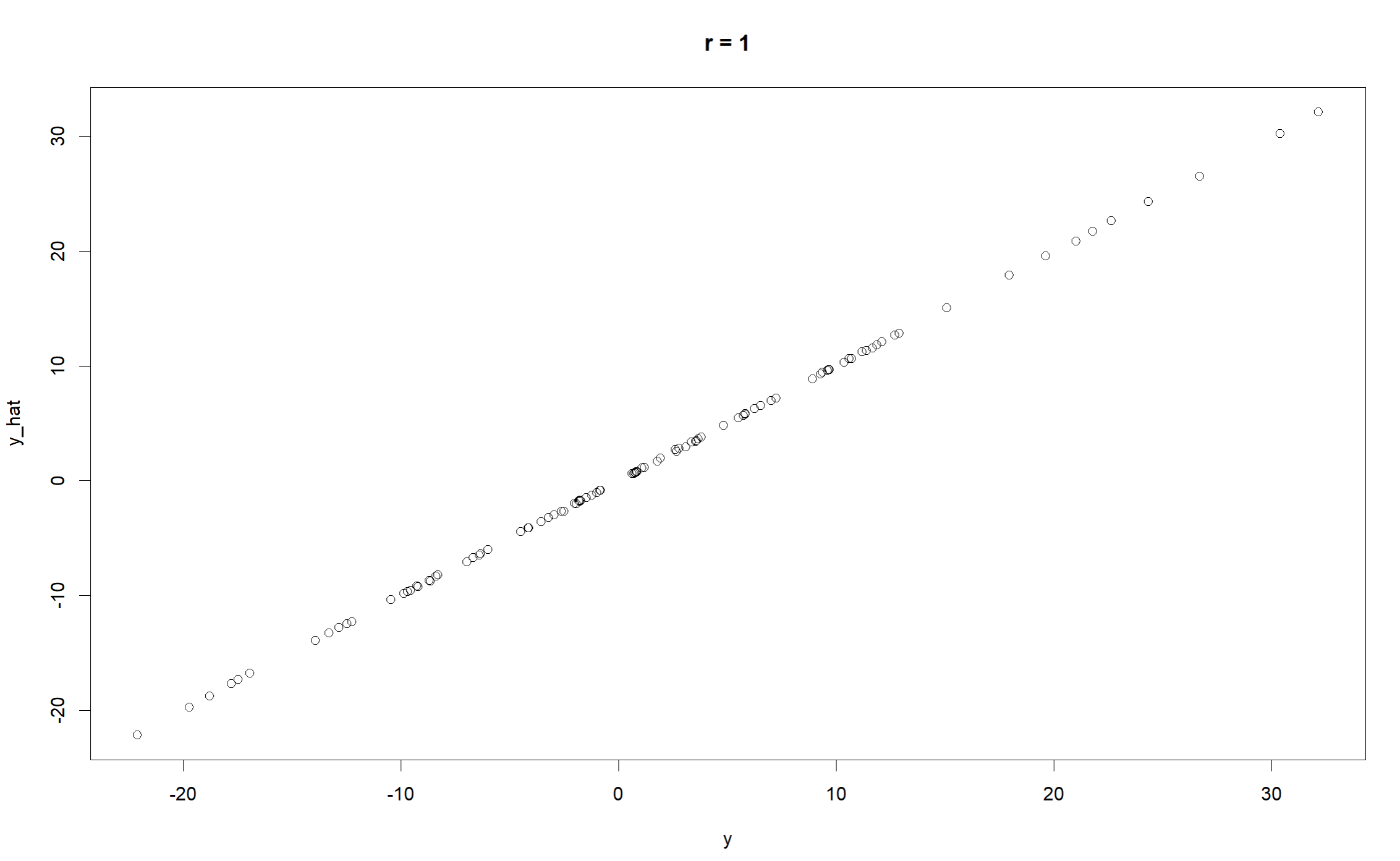
相関の値はかなり高い。上手くパラメータの推定ができているようだ。
また、マーカー効果の分散（$\sigma_w^2$）、誤差分散（$\sigma_e^2$）の推定値の遷移についても可視化してみる。

sigma_w2_chain <- fit_brr$sigma_w2_samples   # マーカー分散
sigma_e2_chain <- fit_brr$sigma_e2_samples   # 誤差分散

n_save <- length(sigma_w2_chain)
iter_index <- seq_len(n_save)  # 保存されたサンプル番号（= 近似的なiteration軸）

# マーカー分散のトレース
plot(iter_index, sigma_w2_chain, type = "l",
     xlab = "Saved iteration index",
     ylab = expression(sigma[w]^2),
     main = paste0("True sigma_w^2 = ", round(sigma_w_true, 2)))
abline(a = sigma_w_true, b = 0, col = "red")

# 誤差分散のトレース
plot(iter_index, sigma_e2_chain, type = "l",
     xlab = "Saved iteration index",
     ylab = expression(sigma[e]^2),
     main = paste0("True sigma_e^2 = ", sigma_e_true))
abline(a = sigma_e_true, b = 0, col = "red")

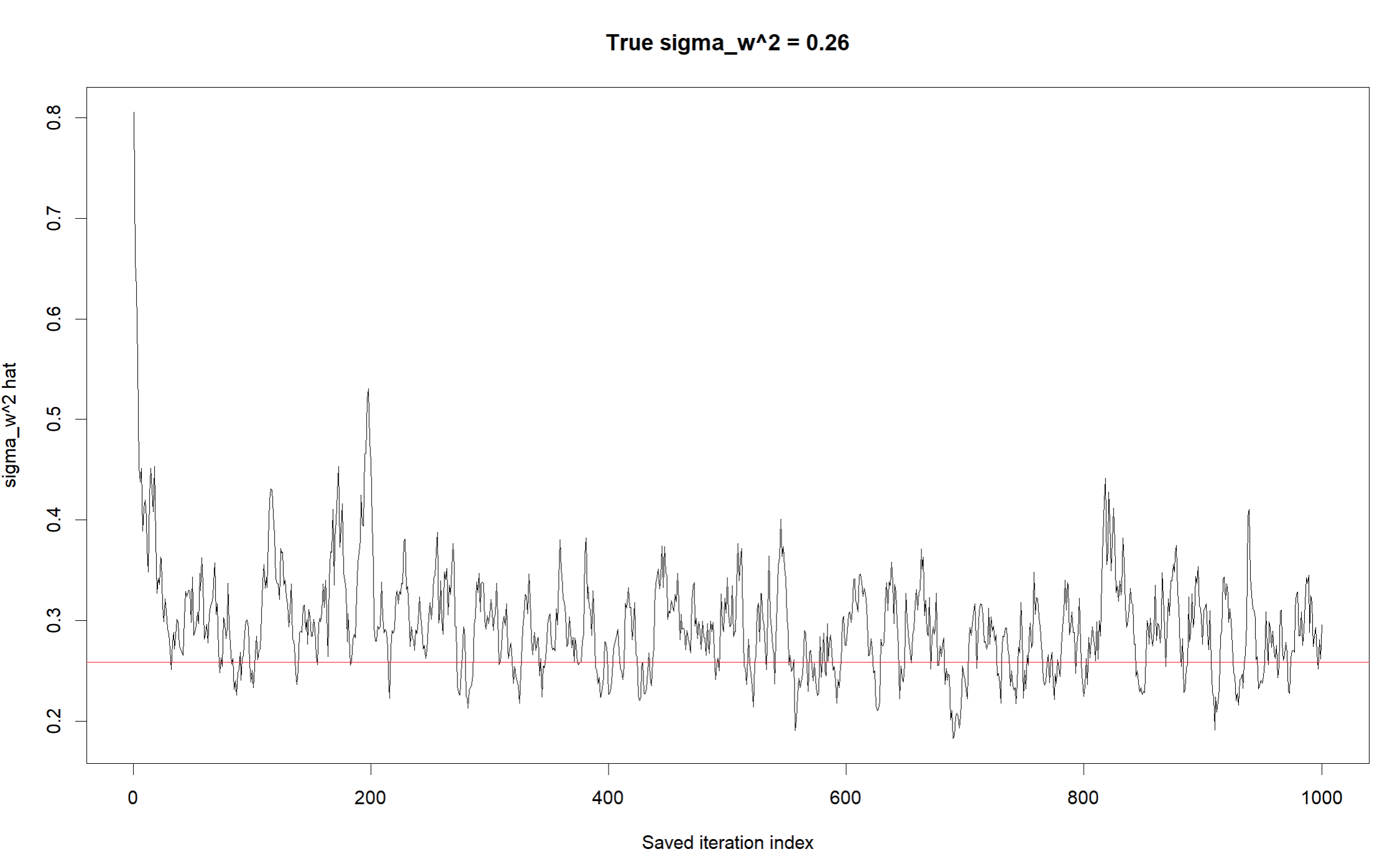
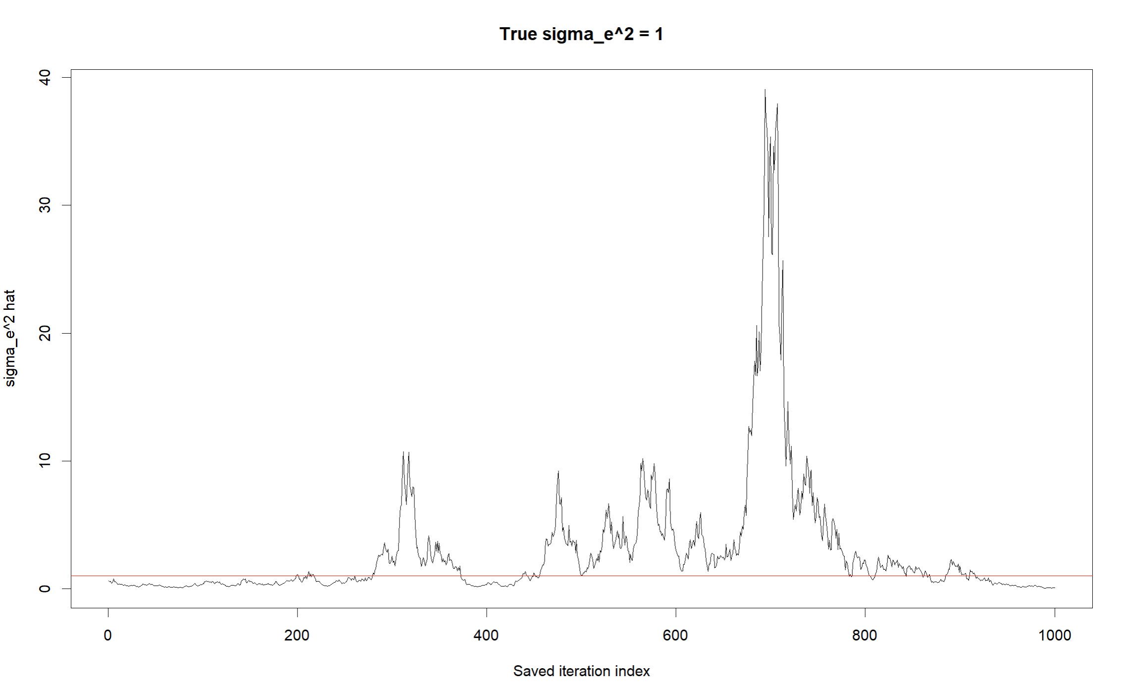
ある程度マーカー効果の分散（$\sigma_w^2$）、誤差分散（$\sigma_e^2$）の両者について正しく推定できているようである。ちなみに上記のコードは驚くほど遅いので注意する。数式を正確に追うために毎回XtX <- crossprod(X) やXty <- crossprod(X, y)の計算を行っている。実際のパッケージBGLRはおそらく高速化を実現するための様々な工夫がなされているのであろう。今回は数式を追うことができたので、ひとまず良しとする。