概要

異常検知(Anomaly detection)について調べていて発見した副産物について書き残そう。
結局オーソドックスなVAEでいくことにしたのだが、このGMMの方がセンスが良く感じる。
DNNを使ったときの手抜き感は小生だけだろうか？

実施期間: 2021年5月
環境：Google Colaboratory
パケージ：scikit-learn

なお、日本語で「異常」というとabnormalのイメージがあるが、abnormalとanomalyはニュアンスが違うので、職場では「異常」という言葉は使わないようにしている。

【変更履歴】
2021/9/4 尤度スコアで等高線を追加した。

モチベーション

Anomaly detectionについて調査中、GaussianMixture Model(GMM)についてのブログを見つけた。
クラスタリングの一種だがK-MeansのようにDeterministicに距離でクラスタ分けするようなアルゴリズムではなく、各点がどのようなGaussian分布に属すべきかをEM(Expectation maximization)で最尤推定するものらしい。
教科書にしているO'REILLYのHands-onでも詳しく説明されており、面白かったので少し味見してみることにした。

以下の順に備忘録として残す。

準備
K-Meansによるクラスタリングの復習
GMMによるクラスタリング
GMMによるクラスタリング数のもとめ方
GMMによるAnomaly Detection

1. 準備

いつもimportしているパケージから取捨選択

import numpy as np
import pandas as pd
import matplotlib.pyplot as plt
from sklearn.datasets import load_iris
from sklearn import metrics
from sklearn import linear_model
from sklearn.metrics import plot_confusion_matrix
from IPython.core.debugger import Pdb # 念のため

今回使用するdatasetはみんな大好きアヤメちゃん

iris = load_iris()
feature_names = iris.feature_names
target_names = iris.target_names

df_iris = pd.DataFrame(data = np.c_[iris['data'], iris['target']],
                     columns = iris['feature_names'] + ['target'])

X = df_iris[['sepal length (cm)', 'sepal width (cm)', 'petal length (cm)', 'petal width (cm)']]
y = df_iris['target']

x_train = np.array(df_iris[['petal width (cm)','petal length (cm)']])
#x_train = np.array(df_iris[['sepal length (cm)', 'sepal width (cm)']])
y_test = np.array(df_iris['target'])

color_codes = {0:'r', 1:'g', 2:'b'}
colors_pred = [color_codes[x] for x in y_test]
plt.scatter(x_train[:,0], x_train[:,1], c=colors_pred)

また、評価結果用の関数を定義

def print_evaluate(x_train, y_test, y_pred, ave='macro'):
    print('accuracy = \t', metrics.accuracy_score(y_true=y_test, y_pred=y_pred))
    print('precision = \t', metrics.precision_score(y_true=y_test, y_pred=y_pred, average=ave))
    print('recall = \t', metrics.recall_score(y_true=y_test, y_pred=y_pred, average=ave))
    print('f1 score = \t', metrics.f1_score(y_true=y_test, y_pred=y_pred, average=ave))
    print('confusion matrix = \n', metrics.confusion_matrix(y_true=y_test, y_pred=y_pred))

※2値のときは average='binary'

2. K-Meansによるクラスタリング

色々とアルゴリズムはあるけれど、GMMで少し言及するK-Meansについて復習する。
簡単に言えば点群の集まりの中心(centroid)がどこかを探すやつ。
指定数のcentroidと全sampleの距離が小さくなるように全centroidを移動させ、収束したときの各centroidに近いsampleがそのクラスタに属するとするアルゴリズム
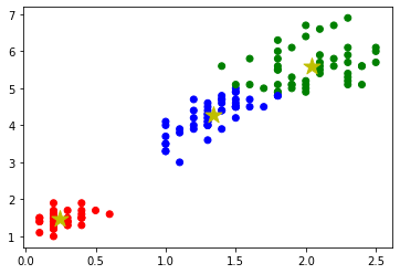
まず、オーソドックスなK-Meansを見てみる。クラスタ(centroid)数は既知のn_clusters=3とする。

from sklearn.cluster import KMeans
from sklearn.cluster import MiniBatchKMeans

## K-Means
kmeans = KMeans(n_clusters=3, random_state=0).fit(x_train)
y_pred = kmeans.labels_
y_cent = kmeans.cluster_centers_

# 精度評価結果
print_evaluate(x_train, y_test, y_pred, 'macro')

colors_pred = [color_codes[x] for x in y_pred]
plt.scatter(x_train[:,0], x_train[:,1], c=colors_pred)
plt.scatter(y_cent[:,0], y_cent[:,1], s = 250, marker='*',c='y')
plt.show

accuracy = 0.37333333333333335
precision = 0.37286324786324787
recall = 0.37333333333333335
f1 score = 0.3730825663598773
confusion matrix =
[[50 0 0]
[ 0 2 48]
[ 0 46 4]]

Confusion matrixで分かるように青と緑はデータがかぶっているため誤判定がみられる。

ついでにMini Batch K-Meansも見てみる。
K-Meansを使うと計算コストが問題になるほどデータ数が多いときに代用するアルゴリズム
任意の数(mini batch)のSampleでK-Means同様にcentroidを移動させるが、mini batchを変えるたびに過去のcentroidと平均する。
精度はK-Meansより劣化するが無視できるほどらしい。

## Mini Batch K-Means
mb_kmeans = MiniBatchKMeans(n_clusters=3, random_state=0, batch_size=6).fit(x_train)
y_pred = kmeans.labels_
y_cent = kmeans.cluster_centers_

# 精度評価結果
print_evaluate(x_train, y_test, y_pred, 'macro')

colors_pred = [color_codes[x] for x in y_pred]
plt.scatter(x_train[:,0], x_train[:,1], c=colors_pred)
plt.scatter(y_cent[:,0], y_cent[:,1], s = 250, marker='*',c='y')
plt.show

accuracy = 0.37333333333333335
precision = 0.37286324786324787
recall = 0.37333333333333335
f1 score = 0.3730825663598773
confusion matrix =
[[50 0 0]
[ 0 2 48]
[ 0 46 4]]

もともとデータ数が少ないので精度が悪化はわからない。

3. GMMによるクラスタリング

では、まずGaussian Mixture Model (GMM)でK-Meansのようにクラスタリングする。
最初にTrainingを行い、GMMはProbablistic ModelなのでPredictする。
もう少し言うと、predict()はラベルの予測を行い、predict_prob()はそのラベルとなる確率を出力する。
K-Meansはユークリッドな距離でクラスタ分けを行うので確率の概念がなかった。
GMMではこの確率を用いて後述のAnomly ditectionを行うこととなる。
まずモデルを作成する。

from sklearn.mixture import GaussianMixture

## Gaussian Mixture Model
gm = GaussianMixture(n_components=3, n_init=10)
gm.fit(x_train)

# fit()で収束したか確認
print(f'Convergence: {gm.converged_}')

y_pred = gm.predict(x_train)
y_pred = np.array(y_pred, dtype=np.float)  # Predict()の戻りの型がy_testと違うので一応合わせる。
y_pred_prob = gm.predict_proba(x_train)

# 精度評価結果
print_evaluate(x_train, y_test, y_pred, 'macro')

# 共分散行列
print('Covariance matrix = \n', gm.covariances_)

Convergence: True
accuracy = 0.02
precision = 0.019230769230769232
recall = 0.02
f1 score = 0.0196078431372549
confusion matrix =
[[ 0 50 0]
[ 1 0 49]
[47 0 3]]
ラベルの誤判定がK-Meansと比べ、2か所改善していることがわかる。

Covariance matrix =
[[[0.07200287 0.04402642]
[0.04402642 0.30034404]]
[[0.01088496 0.00594793]
[0.00594793 0.02955684]]
[[0.04585075 0.08489919]
[0.08489919 0.24667113]]]
n_components=3で指定したので3クラスタそれぞれの共分散行列（x_trainは2次元なので2行2列）を表示した。
おそらく、標準偏差、共分散ともに小さな真ん中の行列が、分布が比較的集中している緑のアヤメを示していると思う。

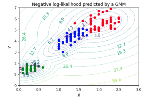
gm.score_samplesで等高線を追加した。

colors_pred = [color_codes[x] for x in y_pred]

# https://scikit-learn.org/stable/auto_examples/mixture/plot_gmm_pdf.html#sphx-glr-auto-examples-mixture-plot-gmm-pdf-py
x = np.linspace(0., 3.)
y = np.linspace(0., 7.)
X, Y = np.meshgrid(x, y)
XX = np.array([X.ravel(), Y.ravel()]).T
Z = -gm.score_samples(XX)
Z = Z.reshape(X.shape)

cont = plt.contour(X, Y, Z, norm=LogNorm(vmin=1.0, vmax=100.0),
                    levels=np.logspace(0, 3, 20), 
                    linestyles='dashed', linewidths=0.5)

cont.clabel(fmt='%1.1f', fontsize=12)
plt.xlabel('X', fontsize=12)
plt.ylabel('Y', fontsize=12)

plt.title('Negative log-likelihood predicted by a GMM')
plt.scatter(x_train[:,0], x_train[:,1], c=colors_pred)
plt.show

4. GMMによるクラスタ数のもとめ方

クラスタごとのGaussian disributionを現すパラメータは少なければ少ないほどよく、一方そのパラメータのlikelihood（尤度）は大きければ大きいほどよい。
とてもおおざっぱだけど、それを表現する基準がBIC(Bayesian Information Criterion)とAIC(Akaike Information Criterion)である。
詳細は上述Hands-on教科書のP267~269に解説あり。
クラスタ数を振ってBIC, AICをプロットすると最適なクラスタ数を得ることができる。

n_components = np.arange(1, 10)
models = [GaussianMixture(n, n_init=10).fit(x_train)
         for n in n_components]

fig, ax = plt.subplots(figsize=(9,7))
ax.plot(n_components, [m.bic(x_train) for m in models], label='BIC')
ax.plot(n_components, [m.aic(x_train) for m in models], label='AIC')

plt.legend(loc='best')
plt.xlabel('n_components')

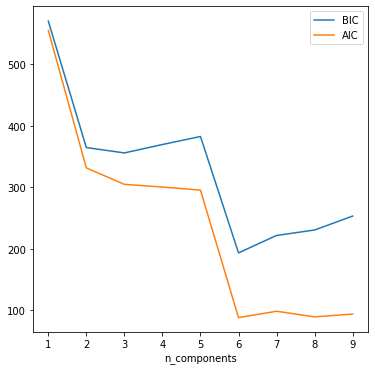
ゑっ？　よく見るチャートぢゃない・・・

サンプル数150が少ないのかもしれない。
GMMはProbabilistic modelなのでsample()メソッドで確率密度に沿ったデータの増産することができる。
そこで合計1000個(+850個)まで増やして再描画してみる。

x_new, y_new = gm.sample(850)
x_new = np.array(x_new).reshape(850,2)
y_new = np.array(y_new)
x_augment = np.vstack([x_train, x_new])
y_augment = np.append(y_test, y_new)

n_components = np.arange(1, 10)
models = [GaussianMixture(n, n_init=10).fit(x_augment)
         for n in n_components]

fig, ax = plt.subplots(figsize=(6, 6))
ax.plot(n_components, [m.bic(x_new1) for m in models], label='BIC')
ax.plot(n_components, [m.aic(x_new1) for m in models], label='AIC')

plt.legend(loc='best')
plt.xlabel('n_components')

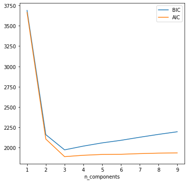
3の時がBIC,AICともに最小であることから、クラスタ数=3が尤もらしいとわかる。
（よかった）

もちろんK-Meansでもsilhouette_score()やsilhouette diagramで最適なクラスタ数を推定することができる。

5. GMMによるAnomaly Detection

調べたいデータがanomalyか否かは上述のGMMモデルのスコアとしてscore_samples()で簡単に調べることができる。
これで得られるスコアはデータの確率密度の濃さを示している。
なお、scikit-learnのscore_samples()は自然対数で返すためexp()した。

例えばデータ群の中の(0.2, 0.1)とデータ群から外した(2.5, 0.5)の２データについてスコアを見てみる。

x_compare = np.array([0.2, 1.0, 2.5, 0.5]).reshape(2, 2)
print(x_compare)

score_compare = gm.score_samples(x_compare)
print(np.exp(score_compare))

[[0.2 1. ]
[2.5 0.5]]
[7.56273077e-02 1.36493463e-24]

期待通り、前者が大きくなり、後者はほぼゼロとなっている。データ分布がGaussianなら色々使えそう。
もちろん、特異点の判断基準はドメインの要求によるため言及できない。

以上

GaussianMixture modelによる異常検知 備忘録

概要