要点
-
@harmegiddoさんの以下の記事をもとに、トロッコ問題を例としたカルマンフィルタを実装していました(勉強のため)
- 【カルマンフィルタの実装と理論】トロッコ問題で理解するカルマンフィルタ (実装済み)
- 予測分布とフィルタ分布の精度差を見るための改変もしました。
- カルマンフィルタは線形ガウス状態空間モデルを前提としています。
- 非線形な状態方程式が蔓延るこの世に対応するために、状態方程式が線形ガウスでなくても適用できるアンサンブルカルマンフィルタなる代物が開発されています。
- 詳しい話は@g_rej55さんの以下の記事とか読めばいいと思います。
- トロッコ問題の状態方程式は線形ガウスですが、せっかくなので勉強のためにアンサンブルカルマンフィルタをぶち込んでみました。
- ついでにアンサンブルメンバ数と推測精度の関係も検討してみました。
実行結果(コードは記事の最後です)
フィルタ分布と予測分布の推定精度の比較
アンサンブルメンバ数は100での試行の一例です。
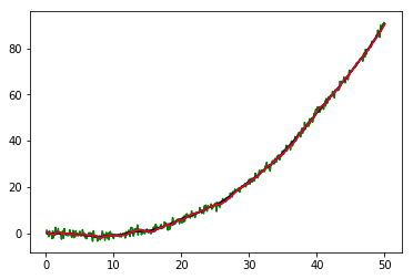
横軸が時間、縦軸がトロッコの位置です。
また、緑が観測、黒が真値、青が予測分布のアンサンブル近似に基づく推定値、赤がフィルタ分布のアンサンブル近似に基づく推定値です。
これだけだとよくわからないので、真値に対する差も比べてみましょう。緑が観測と真値の差、青が予測分布のアンサンブル近似に基づく推定値と真値の差、赤がフィルタ分布のアンサンブル近似に基づく推定値と真値の差です。
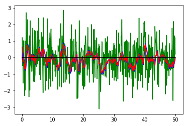
青線と赤線を比べると、赤線の方がより小さい差となっていることがわかります。
つまり、観測前の予測分布アンサンブル近似に基づく推定値より、観測情報を加味したフィルタ分布アンサンブル近似に基づく推定値の方が精度が良い、ということですね。
MSEの比較もしてみましょう。
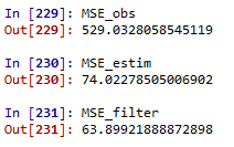
やったぜ。
アンサンブルメンバ数の違いによる推定精度の差異
これだけだと前回の記事そのまんまなので、今回はアンサンブルによる手法らしく、アンサンブルメンバ数による推定精度の違いも見てみます。
アンサンブルメンバ数10、100、1000でそれぞれ10000回トロッコ問題を走らせ、観測、予測分布アンサンブル近似、フィルタ分布アンサンブル近似それぞれのMSEの分布をバイオリンプロットにしてみました。
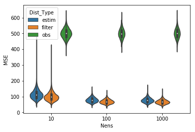
さすがにメンバ数10とそれ以外では改善に大きな差がありますね。観測を省いてみましょう。
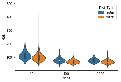
うーむ、やっぱりメンバ数100と1000ではあまり変わっていないように見えます。
フィルタ後のMSEに関する10000試行の平均値を見てみましょう。上からメンバ数10, 100, 1000です。
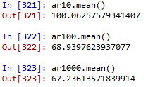
メンバ数100と1000ではそこまで推定精度が変わりませんね。ノイズの大きさやモデルそのものなどいろいろ要因はありそうですが、これくらいがEnKFによるトロッコ問題の推定精度の限界っぽいです。
コード
以下のコードはほとんど@harmegiddoさんのコードをベースにしています。大感謝祭。
# implementation of Ensemble Kalman Filter for Truck problem
# https://qiita.com/g_rej55/items/618778dbb4bf286a985b

import numpy as np
import numpy.random as random
import matplotlib.pyplot as plt

# generate norm
def norm(_loc=0.0, _scale=1.0, _size=(1)):
	return random.normal(_loc, _scale, _size)

# --------------------------------------------------------- #
# universal setting
# --------------------------------------------------------- #

# time
global_time = 0
# set dt
dt = 0.1
# calc setting
calc_num = 500
end_time = calc_num * dt

# unit matrix
I = np.matrix([
				[1, 0],
				[0, 1]
			])

# --------------------------------------------------------- #
# physical equations and settings
# --------------------------------------------------------- #
# kinematic equation
F = np.matrix([
				[1, dt],
				[0, 1]
			])

# external force to state vector matrix
B = np.matrix([
				[(dt**2) / 2],
				[dt]
			])

# external force component
f = np.array([0.01]) # hyp. of constant external force

# noize to state vector matrix (accidential acceralation)
G = np.matrix([
				[(dt**2) / 2],
				[dt]
			])

# system noize parametres : v_t ~ N(mean_v, sigma_v)
mean_v = 0 # if dim(v_t) > 1, it becomes vector
sigma_v = 1 # if dim(v_t) > 1, it is co-var mtx.

# system noize covariance mtx
# note: cov = sigma**2 * G * G.T in the original article
# but because v_t is 1 dim, Q = sigma_v**2, not a co-ver mtx.
Q = (sigma_v**2)

# --------------------------------------------------------- #
# observation equations
# --------------------------------------------------------- #
# obs matrix
H = np.matrix([
				1,
				0
			])

# obs noize : w_t ~ N(mean_w, sigma_w)
mean_w = 0 # if dim(w_t) > 1, it becomes vector
sigma_w = 1 # if dim(w_t) > 1, it becomes co-var mtx

# obs error covariance mtx or scalar
R = (sigma_w**2)


# --------------------------------------------------------- #
# set initial condition
# --------------------------------------------------------- #

# initial state vector
# note: ave and covmtx of x0/0 is known
x_true_t = np.matrix([
					[0],
					[0]
				])

y_t = H * x_true_t + norm(mean_w, sigma_w)

# estimated dist of 1/0 can be calc.d from init cond.
x_ave_t_t = np.matrix([
						[0],
						[0]
					])

V_t_t = np.matrix([
					[0, 0],
					[0, 0]
				])

# for plotting
li_xtrue = []
li_obs_yt = []
li_estim_xavett1 = []
li_filter_xavett = []
li_t = []

# --------------------------------------------------------- #
# set initial ensemble members and ensemble conditions
# --------------------------------------------------------- #

N_ens = 100
li_x_ensmem = [np.matrix([norm(0.0, 1.0),norm(0.0, 1.0)]) for i in range(N_ens)]
X_ens_t_t = np.concatenate(li_x_ensmem, axis = 1)

One_N = np.matrix([[1.0 for i in range(N_ens)] for j in range(N_ens)])

I_ens = np.matrix(np.identity(N_ens))

# --------------------------------------------------------- #
# actual calculation
# --------------------------------------------------------- #

while global_time < end_time:

	# 0. time count
	global_time += dt
	li_t.append(global_time)

	# 1. renew the x_true_t
	v_t = norm(mean_v, sigma_v)
	# x_true_t = F * x_true_t + G * v_t # w/o external force f
	x_true_t = F * x_true_t + G * v_t + B * f # with external force f
	li_xtrue.append(x_true_t.tolist()[0][0])

	# 2. renew ensemble members for t based on t-1 info
	#    and calculate t/t-1 estimation distribution approximated with ensemble
	mtx_vens = np.concatenate([np.matrix([norm(mean_v, sigma_v)]) for i in range(N_ens)], axis = 1)
	mtx_f = np.concatenate([np.matrix(f) for i in range(N_ens)], axis = 1)
	X_ens_t_t1 = F * X_ens_t_t + G * mtx_vens + B * mtx_f
	X_ave_t_t1 = (1/N_ens) * X_ens_t_t1 * One_N
	X_dif_t_t1 = X_ens_t_t1 - X_ave_t_t1
	V_ens_t_t1 = (1/(N_ens-1)) * X_dif_t_t1 * X_dif_t_t1.T
	li_estim_xavett1.append(X_ave_t_t1[0,0]) # ave of x0 of all ens members

	# 3-1. actual observation
	w_t_actual = norm(mean_w, sigma_w)
	y_t = H * x_true_t + w_t_actual
	li_obs_yt.append(y_t.tolist()[0][0])
	Y_t = np.concatenate([y_t for i in range(N_ens)], axis = 1)

	# 3-2. imaginal observation for ensemble members
	W_ens_t = np.concatenate([np.matrix([norm(mean_w, sigma_w)]) for i in range(N_ens)], axis = 1)
	W_ave_t = (1/N_ens) * W_ens_t * One_N
	W_dif_t = W_ens_t - W_ave_t
	R_t = (1/(N_ens-1)) * W_dif_t * W_dif_t.T

	# 4. renew the ensemble members for t based on obs info y_t
	#    and calculate filter dist. as appproximation with ensemble
	Z_t = (I_ens + X_dif_t_t1.T * H.T \
				* np.linalg.inv(H * X_dif_t_t1* X_dif_t_t1.T * H.T \
								+ W_dif_t * W_dif_t.T) \
				* (Y_t + W_dif_t - H * X_ens_t_t1))
	# I do not calculate Kalman Gain explicitly. Please do not throw me a hatchet.
	X_ens_t_t = X_ens_t_t1 * Z_t
	X_ave_t_t = (1/N_ens) * X_ens_t_t * One_N
	li_filter_xavett.append(X_ave_t_t[0,0])

# --------------------------------------------------------- #
# results
# --------------------------------------------------------- #

arr_dif_btw_obs_true = np.array(li_obs_yt) - np.array(li_xtrue)
arr_dif_btw_estim_true = np.array(li_estim_xavett1) - np.array(li_xtrue)
arr_dif_btw_filter_true = np.array(li_filter_xavett) - np.array(li_xtrue)

MSE_obs = np.sum((np.array(li_obs_yt) - np.array(li_xtrue))**2)
MSE_estim = np.sum((np.array(li_estim_xavett1) - np.array(li_xtrue))**2)
MSE_filter = np.sum((np.array(li_filter_xavett) - np.array(li_xtrue))**2)

# if EnKF is effective, it should be like MSE_obs > MSE_estim > MSE_filter

# EOF.
参考文献
樋口知之編著「データ同化入門(シリーズ予測と発見の科学6)」