quiverでの座標軸の取り方

はじめに

quiverと2次元イメージデータと合わせて表示する際に、ちょっと混乱したので、理解のために整理した結果をその覚えとして記載します。

2次元イメージデータの表示（imshow()）では左上が原点のデフォルトとなります。
quiverでは左下が原点のデフォルトになります。
matplotlib.pyplot.quiver
2次元の座標の取り方についてはこちらの記事が参考になります。
N行N列のnumpy arrayを扱う際に気をつけるべき方向と座標の定義

image画像と重ねる場合
（1）imageデータに合わせる場合は、quiverの上下を反転させる。
（2）quiverのデフォルトに合わせる場合は、imageデータの原点を左下にします。
（1）の場合は、quiverに指定するyの値にマイナスをつける必要があります。また、x軸は同じですがy軸は下向きの方向となります。
（2）の場合は、今まで見ていた画像と異なるので違和感がありますが、原点が左下になりy軸が上向きになります。

それぞれ表示の例を以下に示します。
なお、quiverやMatplotlibについては下記のサイトを参考にしました。
python : matplotlib矢筒を画像
plt.subplots()の使い方
matplotlibでAxesを真っ白にする（x軸とかy軸なんかを消して非表示にする）

表示例

import numpy as np
import matplotlib.pyplot as plt

# 　5行5列のx,yの行列をいくつか作成します。

xx = np.array([[1,1,0,-1,-1],[1,1,0,-1,-1],[1,1,0,-1,-1],[1,1,0,-1,-1],[1,1,0,-1,-1]])
yy =np.array([[-1,-1,-1,-1,-1],[-1,-1,-1,-1,-1],[0,0,0,0,0],[1,1,1,1,1],[1,1,1,1,1]])

x1 =np.array([[1,1,1,1,1],[0,0,0,0,0],[1,1,1,1,1],[0,0,0,0,0],[1,1,1,1,1]])
y1= np.array([[1,1,0,-1,-1],[1,1,0,-1,-1],[1,1,0,-1,-1],[1,1,0,-1,-1],[1,1,0,-1,-1]])

xin = np.array([[1,1,0,-1,-1],[1,1,0,-1,-1],[1,1,0,-1,-1],[1,1,0,-1,-1],[1,1,0,-1,-1]])
yin = np.array([[1,1,1,1,1],[1,1,1,1,1],[0,0,0,0,0],[-1,-1,-1,-1,-1],[-1,-1,-1,-1,-1]])

xout = np.array([[-1,-1,0,1,1],[-1,-1,0,1,1],[-1,-1,0,1,1],[-1,-1,0,1,1],[-1,-1,0,1,1]])
yout = np.array([[-1,-1,-1,-1,-1],[-1,-1,-1,-1,-1],[0,0,0,0,0],[1,1,1,1,1],[1,1,1,1,1]])

# xin,yin：矢印が内向きを表示しています。
# 原点が左上の場合です。quiverのyの値をマイナスにしてy軸の方向を逆転させます。

fig, ax = plt.subplots(1,3, figsize=(12,4), squeeze=False, tight_layout=True)
fig.suptitle('Normal origin left top ')
im00 = ax[0,0].imshow(xin)
ax[0,0].set_title('x')
fig.colorbar(im00,ax=ax[0,0])
im01 = ax[0,1].imshow(yin)
ax[0,1].set_title('y')
fig.colorbar(im01,ax=ax[0,1])
ax[0,2].quiver(xin,-yin, color='blue')
ax[0,2].invert_yaxis()
ax[0,2].set_title('xy arrow')
plt.show()

​

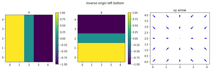
# xin,yin：矢印が内向きを表示しています。
# 原点が左下の場合です。imshowの引数のorigin='lower'とします。

fig, ax = plt.subplots(1,3, figsize=(12,4), squeeze=False, tight_layout=True)
fig.suptitle('Inverse origin left bottom ')
# origin ='lower'
im00 = ax[0,0].imshow(xin,origin='lower')
ax[0,0].set_title('x')
fig.colorbar(im00,ax=ax[0,0])
# origin ='lower'
im01 = ax[0,1].imshow(yin,origin='lower')
ax[0,1].set_title('y')
fig.colorbar(im01,ax=ax[0,1])
# -yy --> yy
ax[0,2].quiver(xin,yin, color='blue')
# ax[0,2].invert_yaxis()
ax[0,2].set_title('xy arrow')
plt.show()

​

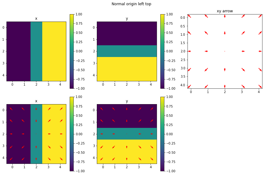
# 先ほどのPlotを何回も書くのが面倒なので関数にします。
def plot_lt(xdata,ydata):
    # 原点左上（Left top)
    fig, ax = plt.subplots(2,3, figsize=(12,8), squeeze=False, tight_layout=True)
    fig.suptitle('Normal origin left top ')
    im00 = ax[0,0].imshow(xdata)
    ax[0,0].set_title('x')
    fig.colorbar(im00,ax=ax[0,0])
    im01 = ax[0,1].imshow(ydata)
    ax[0,1].set_title('y')
    fig.colorbar(im01,ax=ax[0,1])
    ax[0,2].quiver(xdata,-ydata, color='red')
    ax[0,2].invert_yaxis()
    ax[0,2].set_title('xy arrow')

    im10 = ax[1,0].imshow(xdata)
    ax[1,0].set_title('x')
    ax[1,0].quiver(xdata,-ydata, color='red')
    fig.colorbar(im10,ax=ax[1,0])
    im10 = ax[1,1].imshow(xdata)

    im11 = ax[1,1].imshow(ydata)
    ax[1,1].set_title('y')
    ax[1,1].quiver(xdata,-ydata, color='red')
    fig.colorbar(im11,ax=ax[1,1])
    ax[1,2].axis("off")
    plt.show()

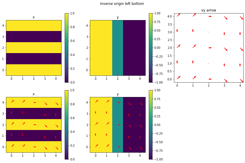
def plot_lb(xdata,ydata):
    # 原点左下（Left bottom)
    fig, ax = plt.subplots(2,3, figsize=(12,8), squeeze=False, tight_layout=True)
    fig.suptitle('Inverse origin left bottom ')
    # origin ='lower'
    im00 = ax[0,0].imshow(xdata,origin='lower')
    ax[0,0].set_title('x')
    fig.colorbar(im00,ax=ax[0,0])
    # origin ='lower'
    im01 = ax[0,1].imshow(ydata,origin='lower')
    ax[0,1].set_title('y')
    fig.colorbar(im01,ax=ax[0,1])
    # -yy --> yy
    ax[0,2].quiver(xdata,ydata, color='red')
    # ax[0,2].invert_yaxis()
    ax[0,2].set_title('xy arrow')

    im10 =ax[1,0].imshow(xdata,origin='lower')
    ax[1,0].set_title('x')
    ax[1,0].quiver(xdata,ydata, color='red')
    fig.colorbar(im10,ax=ax[1,0])
    im10 =ax[1,1].imshow(xdata)

    im11=ax[1,1].imshow(ydata,origin='lower')
    ax[1,1].set_title('y')
    ax[1,1].quiver(xdata,ydata, color='red')
    fig.colorbar(im11,ax=ax[1,1])
    ax[1,2].axis("off")
    plt.show()

plot_lt(xdata=xout,ydata=yout)
plot_lb(xdata=xout,ydata=yout)

​

plot_lt(xdata=x1,ydata=y1)
plot_lb(xdata=x1,ydata=y1)

まとめ

2次元image画像とquiverを重ねる場合
（1）imageデータに合わせる場合は、quiverのyの上下を反転させる（yの値にマイナスをつける。）。Imgae表示がこれまでと同じなので違和感が出ない。
（2）quiverのデフォルトに合わせる場合は、imageデータの原点を左下（imshowの引数のorigin='lower'）にする。物理的な表現（x、y軸の取り方が一般的）をする場合には有効。