0.はじめに
この記事では、ディープラーニングの学習を開始した人が、コード上どのように実装されているのか理解することを目的に、【CNN(Keras)】でのMINIST(手書き数字文字)識別の実装コードを説明します。
CNNがどのような仕組みで実装されているのかの詳細を下記に投稿しています。合わせて参照するとより理解が進むと思います。
1.ネットワークモデル
まず、CNNでMNISTの手書き文字を識別するサンプルコードの全体を見てみましょう。
6   from keras.layers import Dense, Dropout, Flatten, Conv2D, MaxPooling2D
7   # AI_DESIGNER_GEN:IMPORT_BEGIN
8   import keras.backend as K
9   import numpy as np
10  import tensorflow as tf
11  from keras.layers import Input
12  from keras.models import Model
13  # AI_DESIGNER_GEN:IMPORT_END
14
15  # AI_DESIGNER_GEN:MODEL_BEGIN
16
17  def mnist_cnn(input_shape):
18  '''
19  mnist cnn keras
20  @param input_shape input_shape
21  @return  model
22  '''
23
24  # 入力層
25  v_input = Input(shape=input_shape)
26
27  # 畳み込み
28  v_conv2d = Conv2D(filters=32,kernel_size=(3,3),activation='relu')(v_input)
29
30  # 畳み込み
31  v_conv2d1 = Conv2D(filters=64,kernel_size=(3,3),activation='relu')(v_conv2d)
32
33  # 最大値プーリング
34  v_maxpool2d = MaxPooling2D(pool_size=(2,2))(v_conv2d1)
35
36  # ドロップアウト
37  v_dropout = Dropout(rate=0.25)(v_maxpool2d)
38
39  # 平坦化
40  v_flatten = Flatten(data_format=None)(v_dropout)
41
42  # 全結合
43  v_dense = Dense(128,activation='relu')(v_flatten)
44
45  # ドロップアウト
46  v_dropout1 = Dropout(rate=0.5)(v_dense)
47
48  # 全結合
49  v_dense1 = Dense(10,activation='softmax')(v_dropout1)
50
51  # モデル
52  v_model = Model(v_input, v_dense1)
53
54  # 終了
55  return v_model
56  # AI_DESIGNER_GEN:MODEL_END
意外にシンプルですね!!
以下、順を追って説明します。
まず、ハイパーフレームワークであるkerasから、ネットワークを構成する各処理をimportしています。
6 from keras.layers import Dense, Dropout, Flatten, Conv2D, MaxPooling2D
- Dense:全結合処理です(Affine変換やFFNとも呼ばれます)
- Dropout:Dropout処理です
- Flatten:(全結合を行うために)多次元のリストを一次元化します。
- Conv2D:畳み込み処理です
- Maxpooling2D:Max Pooling処理です
各処理の詳細は、CNNの説明を参照してください。
これらの各処理を組み合わせて、後ほどネットワークモデルを構築(生成)します。
次にその他必要なライブラリやクラスをimportします。
8   import keras.backend as K  #kerasのバックエンドを読み出します(今回はTensorflow)
9   import numpy as np #各種ベクトル演算するライブラリィするnumpyの呼び出し
10  import tensorflow as tf  # Tensorflowの呼び出し(直接使うことはありません)
続いてFunctional API型でモデルを生成するためModelをimportします。
11  from keras.layers import Input
12  from keras.models import Model
Inputクラスのインスタンスを作成し入力層を定義します。
shapeは入力の形状になります。 今回はMNISTのデータなので(28, 28, 1)になります。これは、縦=28pixcel、横=**28pixcel、白黒=1**チャネルを表しています。
この後は入力層につなげる形でレイヤを順次記載していきます。
24  # 入力層
25  v_input = Input(shape=input_shape)
入力データの畳み込み「Conv2D」を行います。
3×3の「カーネル(フィルタ)」(kernel_size=(3,3))を32個(filters=32)使って畳み込みます。 また、使用する活性化関数は、「Relu」 (activation='relu')を使用して出力します。
27  # 畳み込み
28  v_conv2d = Conv2D(filters=32,kernel_size=(3,3),activation='relu')(v_input)
そして、この出力を同様にもう一度畳み込み(3×3のカーネルを64個)を行います。
30  # 畳み込み
31  v_conv2d1 = Conv2D(filters=64,kernel_size=(3,3),activation='relu')(v_conv2d)
次にこの2回目の畳み込みに対して最大値プーリング「MaxPooling2D」を行います。
プーリング時のウィンドウサイズは2×2(pool_size=(2,2))です。
34 v_maxpool2d = MaxPooling2D(pool_size=(2,2))(v_conv2d1)
次に、ドロップアウト「Dropout」の定義を行います。
ドロップアウトは過学習を避けるために、学習時に使うニューロンをランダムな比率で選び出して学習される方式です。 今回は25%(rate=0.25)をランダムに消去させて学習します。
37 v_dropout = Dropout(rate=0.25)(v_maxpool2d)
次に、全結合行うためにベクトルを一次元化「Flatten」します。
40 v_flatten = Flatten(data_format=None)(v_dropout)
そして、全結合「DENCE」を行います。
43 v_dense = Dense(128,activation='relu')(v_flatten)
全結合での過学習を防ぐために、再度ドロップアウトの定義を行います。
今回はrate=0.5ですので、50%をランダムに消去して学習します。
46 v_dropout1 = Dropout(rate=0.5)(v_dense)
最後にもう一度全結合を行います。 このとき数字の0~9の10個を予測するため出力数は10にします。 また、活性化関数は「softmax」(activation='softmax')ですが、これは予測した0から9のスコア値がトータル1.0になるように出力します。
49 v_dense1 = Dense(10,activation='softmax')(v_dropout1)
以上が、全体のネットワークモデルになります。
繰り返しになりますが、実装コードはシンプルであることが分かると思います。
さて、ネットワークモデルは定義出来ましたので、次は学習時の実装コードを見てみましょう。
2.学習時の実装コード
6   import datetime
7
8   import keras
9   from keras.datasets import mnist
10  from keras.optimizers import RMSprop
11  from sklearn.model_selection import train_test_split
12
13  from exec_opts import ExecOpts
14  from mnist_cnn_keras import mnist_cnn
15
16
17  def main(epochs=5, batch_size=128):
18      '''
19      MNISTの学習とその結果の表示
20      @args:
21          epochs: epochの回数
22           batch_size: ミニバッチのサイズ
23       '''
24
25      # load MNIST data
26      (x_train, y_train), (x_test, y_test) = mnist.load_data()
27      x_train1, x_valid, y_train1, y_valid = train_test_split(x_train, y_train, test_size=0.175)
28      x_train = x_train1
29      y_train = y_train1
30
31      x_train = x_train.reshape(x_train.shape[0], 28, 28, 1).astype('float32') / 255
32      x_valid = x_valid.reshape(x_valid.shape[0], 28, 28, 1).astype('float32') / 255
33      x_test = x_test.reshape(x_test.shape[0], 28, 28, 1).astype('float32') / 255
34
35      # convert one-hot vector
36      y_train = keras.utils.to_categorical(y_train, 10)
37      y_valid = keras.utils.to_categorical(y_valid, 10)
38      y_test = keras.utils.to_categorical(y_test, 10)
39
40      # create model
41      model = mnist_cnn(input_shape=(28, 28, 1))
42
43      model.compile(loss='categorical_crossentropy',
44                  optimizer=RMSprop(),
45                  metrics=['accuracy'])
46
47      print(model.summary())
48
49      # callback function
50      NAME = "CNN_{}".format(datetime.datetime.now().isoformat(timespec='seconds')).replace(':', '-')
51
52       checkpoint_file_pattern = ExecOpts.get('train', 'checkpoint_file_pattern',
53                                           './checkpoints/weights.{epoch:02d}-{val_loss:.2f}.hdf5')
54
55      # train
56      history = model.fit(x_train, y_train,
57                        batch_size=batch_size, epochs=epochs,
58                        verbose=1,
59                        validation_data=(x_valid, y_valid),
60                        callbacks=[
61                           keras.callbacks.ModelCheckpoint(checkpoint_file_pattern,,
62                                      verbose=1,
63                                      save_weights_only=True),
64                            keras.callbacks.TensorBoard(
65                                log_dir="logs/{}".format(NAME),
66                                histogram_freq=1,
67                                write_images=True)
68                        ])
69
70      weight_file_path = ExecOpts.get('train', 'weight_file_path',
71                                    'mnist_cnn_weights.hdf5')
72      model.save_weights('mnist_cnn_weights.hdf5')
73      model.save("mnist_cnn_graph.hdf5")
74
75      # result
76      score = model.evaluate(x_test, y_test, verbose=0)
77      print('Test loss: {0}'.format(score[0]))
78      print('Test accuracy: {0}'.format(score[1]))
79
80
81  if __name__ == '__main__':
94      epochs = ExecOpts.get('train', 'epoch_num', 5)
95      batch_size = ExecOpts.get('train', 'batch_size', 128)
96
97      main(epochs, batch_size)
まずは、importする主なライブラリィです。
train_test_splitは、データを学習用とテスト用に分離する処理です(デフォルトでは75%が学習用、25%がテスト用)。
11 from sklearn.model_selection import train_test_split
minstの手書き数字文字のデータセットを利用します。
14 from mnist_cnn_keras import mnist_cnn
train.pyを起動するとまず下記コードが実行されます。 オプション情報からエポック数とバッチサイズを取得し(デフォルトはそれぞれ5と128です)、続いてmain(epochs, batch_size) でmain()メソッドを呼び出します。
81  if __name__ == '__main__':
94      epochs = ExecOpts.get('train', 'epoch_num', 5)
95      batch_size = ExecOpts.get('train', 'batch_size', 128)
96
97      main(epochs, batch_size)
main()ではまずmnistのデータをロード(mnist.load_data())します。xは手書き文字画像、yは正解値のラベル(0~9)です。 さらに、学習データを検証用に17.5%分離(x_valid, y_valid)しています。
26     (x_train, y_train), (x_test, y_test) = mnist.load_data()
27      x_train1, x_valid, y_train1, y_valid = train_test_split(x_train, y_train, test_size=0.175)
28      x_train = x_train1
29      y_train = y_train1
入力画像の値を255で割って0.0-1.0の範囲にノーマライズします。
31      x_train = x_train.reshape(x_train.shape[0], 28, 28, 1).astype('float32') / 255
32      x_valid = x_valid.reshape(x_valid.shape[0], 28, 28, 1).astype('float32') / 255
33      x_test = x_test.reshape(x_test.shape[0], 28, 28, 1).astype('float32') / 255
そして、正解ラベルをone-hotベクトルに変換します(10次元のベクトルで正解ラベルのみ1で他は0、ex. 1 = [0, 1, 0, 0, 0, 0, 0, 0, 0, 0] )。
36      y_train = keras.utils.to_categorical(y_train, 10)
37      y_valid = keras.utils.to_categorical(y_valid, 10)
38      y_test = keras.utils.to_categorical(y_test, 10)
モデル定義を生成します。 損失関数には「クロスエントロピー誤差」(categorical_crossentropy)、重みパラメータの更新方法(Optimizer)には「RMSprop」(optimizer=RMSprop())を指定しています。 なお、metrics=['accuracy']は評価関数で平均精度率で評価することを意味しています。
41      model = mnist_cnn(input_shape=(28, 28, 1))
42
43      model.compile(loss='categorical_crossentropy',
44                  optimizer=RMSprop(),
45                  metrics=['accuracy'])
46
47      print(model.summary())
そして、いよいよ学習( model.fit())に入ります。バックプロパゲーションによる重みの補正はフレームワーク内で自動で計算されます。
ここでCallback(Kerasフレームワークから特定の条件を満たされた場合に呼び出されるメソッド)に以下を指定しています。
keras.callbacks.ModelCheckpointは、各Epochの終了時に呼び出されチェックポイントファイルを生成します(生成されるファイル名の形式と、重みのみを保存することを指定しています)。
keras.callbacks.TensorBoardは、Tensorbordのログ出力です(ログ名の形式とヒストグラムをEpoc内で1回作成、またモデルの重みを画像で出力することを指定しています)。
56      history = model.fit(x_train, y_train,
57                       batch_size=batch_size, epochs=epochs,
58                       verbose=1,
59                       validation_data=(x_valid, y_valid),
60                       callbacks=[
61                          keras.callbacks.ModelCheckpoint('checkpoint_file_pattern,
62                                      verbose=1,
63                                      save_weights_only=True),
64                            keras.callbacks.TensorBoard(
65                                log_dir="logs/{}".format(NAME),
66                                histogram_freq=1,
67                                write_images=True)
68                        ])
学習が終わったら、重みとモデルを保存します。
72      model.save_weights('mnist_cnn_weights.hdf5')
73      model.save("mnist_cnn_graph.hdf5")
最後に、検証データを使って評価を行い結果を表示します。
76      score = model.evaluate(x_test, y_test, verbose=0)
77      print('Test loss: {0}'.format(score[0]))
78      print('Test accuracy: {0}'.format(score[1]))
以上が学習時のコードの実装の流れになります。概ね分かったのではないでしょうか?
次にテスト時の実装コードについて説明します。
3 テスト時の実装コード
テスト時の実装コードは以下になっています。主要なロジックは学習時のコードで説明しているので、差分に絞って説明します。
6   import matplotlib.pyplot as plt
7   import numpy as np
8   from keras.datasets import mnist
9   from keras.optimizers import RMSprop
10
11  from exec_opts import ExecOpts
12  from mnist_cnn_keras import mnist_cnn
13
14
15  def main():
16      '''
17      MNISTの学習とその結果の表示
18      @args:
19          epochs: epochの回数
20          batch_size: ミニバッチのサイズ
21      '''
22
23      # load MNIST data
24      (x_train, y_train), (x_test, y_test) = mnist.load_data()
25      x_test = x_test.reshape(x_test.shape[0], 28, 28, 1).astype('float32') / 255
26
27      # create model
28      model = mnist_cnn(input_shape=(28, 28, 1))
29
30      model.compile(loss='categorical_crossentropy',
31                    optimizer=RMSprop(),
32                    metrics=['accuracy'])
33
34      weight_file_path = ExecOpts.get('test', 'weight_file_path',
35                                       'mnist_cnn_weights.hdf5')
36      model.load_weights(weight_file_path)
37
38      # TEST_SIZE = 20
39      TEST_SIZE = ExecOpts.get('test', 'test_sample_size', 20)
40
41      index = np.random.randint(0, x_test.shape[0], TEST_SIZE)
42      x_test_ = x_test[index]
43      # y_test_ = y_test[index]
44
45      y_test_ = model.predict(x_test_)
46
47      fig = plt.figure(figsize=(8, 8))
48      columns = 4
49      rows = (TEST_SIZE + columns - 1) // columns
50
51      for i in range(TEST_SIZE):
52          cls_idx = np.argmax(y_test_[i])
53          # cv2.imshow('img %d class: %d ' % (i, cls_idx), x_test_[i])
54
55          col = i % columns
56          row = i // columns
57          ax = fig.add_subplot(rows, columns, i + 1)
58          ax.set_title('class: %d ' % (cls_idx))
59          ax.set_xticks([])
60          ax.set_yticks([])
61          img = np.squeeze(x_test_[i])
62          plt.imshow(img)
63
64      # cv2.waitKey()
65      plt.show()
66
67
68   if __name__ == '__main__':
76       main()
学習済みモデルをロードします。
36 model.load_weights(weight_file_path)
ランダムにテストデータから20枚を選択します。
39      TEST_SIZE = ExecOpts.get('test', 'test_sample_size', 20)
40
41      index = np.random.randint(0, x_test.shape[0], TEST_SIZE)
42      x_test_ = x_test[index]
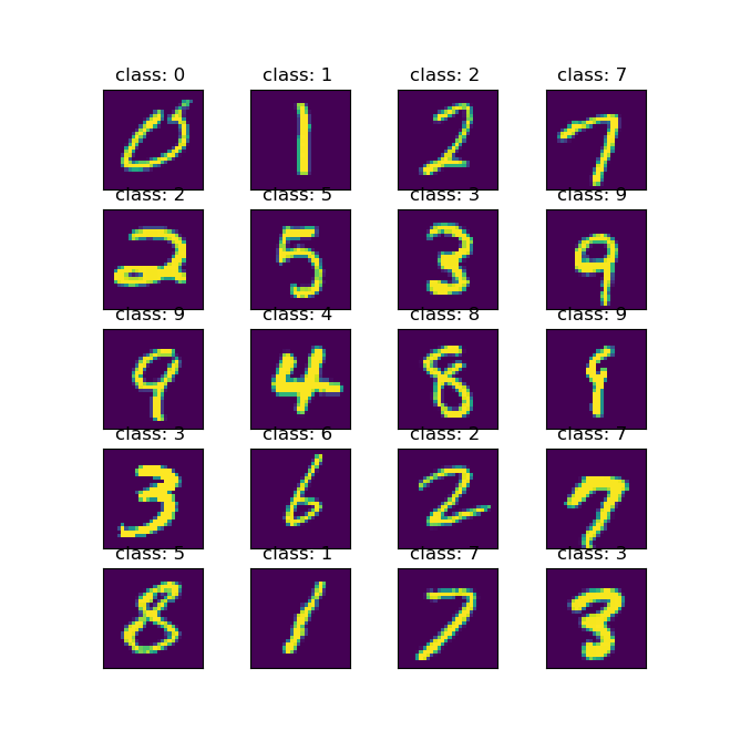
選択したテストデータの予測をします。
45 y_test_ = model.predict(x_test_)
以降の48行目以降のコードで入力した手書き数字文字と予測した結果(数字)を画像で表示します。 表示されるサンプル画像は以下のようになります。
4.おわりに
以上が、MNIST(手書き数字文字)のモデル・学習コード・テストコードになります。
このモデルはディープラーニングの基礎になりますので、ディープラーニングがどのように実装され学習されているのか理解に役立てればと思います。
また、様々なモデルの説明を下記ホームページにも記載しています。
興味がある方は見ていただけると幸いです。