[SIGNATE練習問題]自動車の評価をやってみた#2 〜Metric Learningしてみた〜

前回の試しにXGBoostでやってみた記事から、距離学習を入れてみた。

※前回記事：[SIGNATE練習問題]自動車の評価をやってみた

Label EncodingとOne-hot Encodingの違い

前回はいきなりOne-hot Encodingで、カテゴリ変数化したが
Label Encodingによるカテゴリ変数化でも良いのでは？と思われたかもしれない。
という訳で、今回はまずLabel EncodingとOne-hot Encodingの2つを
検証してみる。

ライブラリを読み込み

#ライブラリインポート
import numpy as np
import pandas as pd
import pandas_profiling as pdpf
import matplotlib.pyplot as plt
from tqdm import tqdm_notebook
import umap
import metric_learn
from scipy.sparse.csgraph import connected_components
from xgboost import XGBRFClassifier
from sklearn.model_selection import train_test_split
from sklearn.preprocessing import LabelEncoder

データ読み込み

#train data
train = pd.read_csv('./train.tsv',sep='\t')
#test data
test = pd.read_csv('./test.tsv', sep='\t')

目的変数と説明変数に分離

#説明変数
train_df = train.drop(['id','class'], axis=1)
#test用の説明変数
test_df = test.drop('id', axis=1)
#目的変数
y = train['class']

#確認
print("train_df:",train_df.shape,
      "y:",y.shape,
      "test_df :",test_df.shape)

TrainとTestを合体

# trainとtestでカテゴリーが異なるとダメだから、trainとtestをマージ
length = train.shape[0]

df = pd.concat([train_df, test_df], axis=0)
print(df.columns)

ようやく本題！

Label Encoding

df_le = pd.concat([train_df, test_df], axis=0)

for i in list(df_le.columns):
    la_en = LabelEncoder()
    print(str(i))
    la_en = la_en.fit(df_le[i])
    la_en.fit(df_le[i])
    df_le[i] = la_en.transform(df_le[i])

train_le = df_le.iloc[:length,:]
test_le = df_le.iloc[length:,:]
display(df_le)

Label Encodingでは、それぞれ'0','1','2','3'などで、ただただカテゴリ変数化される。

	buying	maint	doors	persons	lug_boot	safety
0	1	2	2	0	2	1
1	1	0	2	2	2	2
2	3	0	0	0	2	2
3	0	0	2	2	0	2
4	0	0	2	0	1	0
...	...	...	...	...	...	...
859	1	1	2	0	0	0
860	2	1	0	0	0	2
861	3	3	2	0	0	2
862	0	3	1	1	2	1
863	1	0	2	0	2	0

One-hot Encoding

一方、One-hot表現では、それぞれが[0,0,1],[0,1,0],[1,0,0]のように独立にラベル変数化されることがメリットである。
※ただのLabel Encodingでは、今回の'persons変数では
0:2人、1:4人、2:Moreとなるが、2人とMoreの平均が4人となってしまう。(ってことはMoreは6人??)

この様な独立なラベルは、独立なまま特徴量にしたいからOne-hot Encodingを使う

df_oe = pd.concat([train_df, test_df], axis=0)
df_dummy = pd.get_dummies(df_oe, prefix=df.columns)

train_oe = df_dummy.iloc[:length,:]
test_oe = df_dummy.iloc[length:,:]

display(df_dummy)

目的変数もラベル化

#LabelEncoderのインスタンスを生成
le = LabelEncoder()
#ラベルを覚えさせる
le = le.fit(["unacc", "acc", "good", "vgood"])
#ラベルを整数に変換
y_label = le.transform(y)
y_label_i = le.inverse_transform(y_label)

XGBoostで学習

X_train_le, X_test_le, y_train_le, y_test_le = train_test_split(train_le,y_label,test_size = .2,random_state = 666,stratify = y_label)

X_train_oe, X_test_oe, y_train_oe, y_test_oe = train_test_split(train_oe,y_label,test_size = .2,random_state = 666,stratify = y_label)

import xgboost as xgb
from sklearn.metrics import accuracy_score

#### Label Encoding ####
dtrain = xgb.DMatrix(X_train_le, label=y_train_le,
                     feature_names=X_train_le.columns)
dvalid = xgb.DMatrix(X_test_le, label=y_test_le,
                    feature_names=train_le.columns)
dtest = xgb.DMatrix(test_le,
                    feature_names=train_le.columns)
xgb_params = {
    'objective': 'multi:softmax',
    'num_class': 4,
    'eval_metric': 'mlogloss',
}

evals = [(dtrain, 'train'), (dvalid, 'eval')]
evals_result = {}

bst_le = xgb.train(xgb_params,
                dtrain,
                num_boost_round=100,
                early_stopping_rounds=10,
                evals=evals,
                evals_result=evals_result
                )

#### One-hot Encoding ####
dtrain_oe = xgb.DMatrix(X_train_oe, label=y_train_oe,
                     feature_names=X_train_oe.columns)
dvalid_oe = xgb.DMatrix(X_test_oe, label=y_test_oe,
                    feature_names=train_oe.columns)
dtest_oe = xgb.DMatrix(test_oe,
                    feature_names=train_oe.columns)
xgb_params = {
    'objective': 'multi:softmax',
    'num_class': 4,
    'eval_metric': 'mlogloss',
}

evals = [(dtrain_oe, 'train'), (dvalid_oe, 'eval')]
evals_result = {}

bst_oe = xgb.train(xgb_params,
                dtrain_oe,
                num_boost_round=100,
                early_stopping_rounds=10,
                evals=evals,
                evals_result=evals_result
                )

結果

微々たる差だが、One-hotが優勢っぽい

特徴量増加のためMetric Learningをトライ

微妙な差で勝利したOne-hot版の説明変数を使用。
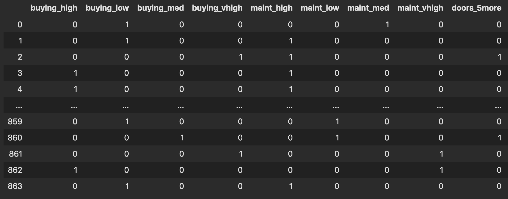
まずは、どんなデータになっているかを次元圧縮によって可視化(UMAPを使用)

%time embedding = umap.UMAP().fit(train_oe)
plt.scatter(embedding.embedding_[:,0],
            embedding.embedding_[:,1],
            c=y_label,
            cmap='plasma')
plt.colorbar()
plt.savefig('./fig/one-hot_umap.png', bbox_inches='tight')
plt.show()

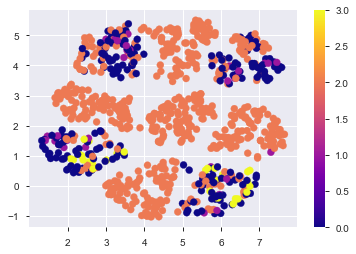
今回は、この変数をscikit-learnのmetric learnを使って次元圧縮。

met_le = metric_learn.LMNN(k=5)
met_le.fit(train_oe, y_label)
%time X_met = met_le.transform(train_oe)
%time X_met_test = met_le.transform(test_oe)

%time met_embedding = umap.UMAP().fit(X_met)
%time test_embedding = met_embedding.transform(X_met_test)

plt.scatter(met_embedding.embedding_[:,0],
            met_embedding.embedding_[:,1],
            c=y_label,
            cmap='plasma')
plt.colorbar()
plt.savefig('./fig/metric_umap.png', bbox_inches='tight')
plt.show()

何もしない時よりも綺麗に分かれてる！気がする。
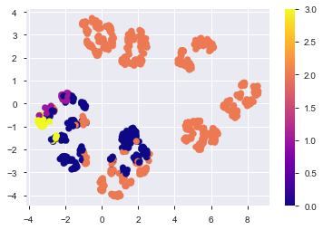
この分布上にTest用のデータを並べてみる。

plt.scatter(met_embedding.embedding_[:,0],
            met_embedding.embedding_[:,1],
            c=y_label,
            cmap='plasma',
            label='train')
plt.colorbar()
plt.scatter(test_embedding[:,0],
            test_embedding[:,1],
            c='gold',
            edgecolor='black',
            linewidth=.7,
            marker='*',
            s=50,
            label='test')
plt.legend()
plt.savefig('./fig/metric_test_on.png', bbox_inches='tight')
plt.show()

これだけでもなんとなく分離できそう...??

座標位置と距離を新たな特徴量として追加

元々のOne-hot encodingの説明変数に、今回作ってみた特徴量を追加。

X_met_df = pd.DataFrame(X_met,
                        columns=np.arange(0,21,1).astype(str))

X_met_test_df = pd.DataFrame(X_met_test,
                             columns=np.arange(0,21,1).astype(str))

embe = pd.DataFrame(met_embedding.embedding_,
                    columns=['locate_x', 'locate_y'])

test_embe = pd.DataFrame(test_embedding,
                         columns=['locate_x', 'locate_y'])

met_oe = pd.concat([train_oe, X_met_df], axis=1)
met_oe = pd.concat([met_oe, embe], axis=1)

met_test_oe = pd.concat([test_oe, X_met_test_df], axis=1)
met_test_oe = pd.concat([met_test_oe, test_embe], axis=1)

print(met_oe.shape, met_test_oe.shape)

# (864, 44) (864, 44)

再度XGBoostで学習

X_train_me, X_test_me, y_train_me, y_test_me = train_test_split(met_oe,
                                                                y_label, 
                                                                test_size = .2,
                                                                random_state = 666,
                                                                stratify = y_label)
dtrain_me = xgb.DMatrix(X_train_me,
                        label=y_train_me,
                        feature_names=X_train_me.columns)
dvalid_me = xgb.DMatrix(X_test_me,
                        label=y_test_me,
                        feature_names=X_train_me.columns)
dtest_me = xgb.DMatrix(met_test_oe,
                       feature_names=met_test_oe.columns)

xgb_params = {
    'objective': 'multi:softmax',
    'num_class': 4,
    'eval_metric': 'mlogloss',
}

evals = [(dtrain_me, 'train'), (dvalid_me, 'eval')]
evals_result = {}

bst_me = xgb.train(xgb_params,
                dtrain_me,
                num_boost_round=100,
                early_stopping_rounds=10,
                evals=evals,
                evals_result=evals_result
                )

ちなみに、特徴量寄与度はこんな感じ

_, ax = plt.subplots(figsize=(12, 8))
xgb.plot_importance(bst_me,
                    ax=ax,
                    importance_type='weight',
                    show_values=True)
plt.show()

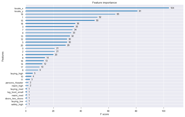
座標位置が効いていそう...

結果出力

y_pred_me = bst_me.predict(dtest_me)
y_pred_me = y_pred_me.astype(np.int)
y_pred_me_i = le.inverse_transform(y_pred_me)

submit_me = pd.read_csv('./sample_submit.csv', sep=',',header=None)
submit_me.loc[:,1] = y_pred_me_i
submit_me.to_csv("test_submit_me.csv", index = None, header = None)

あれ！！！なんか精度下がっている！！
過学習しているのか！？

もう少し真面目に特徴量を増やすのと、過学習防止に5-foldでの検証など
まだまだやる余地はたくさんありそう。

でもMetric Learningによる特徴量生成はうまくいく可能性がありそう。

to be continued.